This post will guide you how to use Excel INDEX function with syntax and examples in Microsoft excel.
Description
The Excel INDEX function returns a value from a table based on the index (row number and column number). You can use INDEX function to extract entire rows or entire columns. This function is used to combine with the MATCH function to lookup value in a range or array.
The INDEX function is a build-in function in Microsoft Excel and it is categorized as a Lookup and Reference Function.
The INDEX function is available in Excel 2016, Excel 2013, Excel 2010, Excel 2007, Excel 2003, Excel XP, Excel 2000, Excel 2011 for Mac.
Syntax
There are two ways to use the INDEX function in excel:
If you want to get the value of a specified cell or array of cell, you can refer to Array form.
If you want to get a reference to specified cells, you can refer to Reference form.
The syntax of the INDEX function is as below:
= INDEX (array, row_num,[column_num])      #Array form
=INDEX(reference, row_num,[column_num],[area_num)     #Reference form
The array form is used in most cases, and if the first argument of the INDEX function is an array constant, you need to use the array form. If you want to perform a three-way lookup in a range, you can use the reference form.
Where the INDEX function arguments are:
- array -This is a required argument. A range of cells or data array. If array contains only one row or column, the corresponding row_num or Column_num argument is optional.
- Row_num – The row number in data array. If Row_num is omitted, column_num is required.
- Column_num – The column position in data array. If Column_num is omitted, row_num is required.
- Area_num – it is set as a number. If the first argument point to more cell ranges, if area_num is set to 1, then the first area will be selected.
Note:
- If you set the row_num and column_num at the same time, the INDEX function will return the value in the cell at the intersection of row number and column number.
- If you set the value of row_num or column_num to 0, the INDEX function will return the array of values for the entire row or column in the array data.
- Row_num and Column_num must point to a cell within array data, if not, the index function returns #REF!
Excel INDEX Function Example
The below examples will show you how to use Excel INDEX Lookup and Reference Function to return a value from a table based on the intersection of row number and column number.
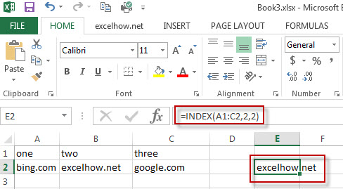
#1 To get the value at the intersection of the second row and second column in the table array: A1:C2, just using the following excel formula:
=INDEX(A1:C2,2,1)
#2 use reference form to extract a value form the second area of C2:D5. Using the following formula.
=INDEX((B1:C5,C2:D5),2,2,2)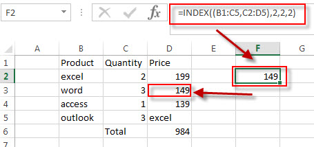
You will see that the intersection of the second row and second column in the second area of C2:D5, which is the contents of cell D3. It returns 149.
More Excel INDEX Formula Examples
- Get the First Match in Two Excel Ranges
If you want to find the first match between two excel ranges, you can use a combination of the INDEX function, the MATCH function and COUNTIF function to create a new formula…. - Extract a List of Unique Values from a Column Range
f you want to extract a list of unique items from a column or range, you can use a combination of the IFERROR function, the INDEX function, the MATCH function and the COUNTIF function to create an array formula….. - Find the Relative Position in a Range or Table
If you want to know the relative row position for all rows in an Excel Range (B3:D6), you can use a excel Array formula as follows:=ROW(B3:D6)- ROW(B3) + 1. You can also use another excel array formula to get the same result as follows:=ROW(B3:D6)-ROW(INDEX(B3:D6,1,1))+1… - Get the Last Row Number in a Range
If you want to get the last row number in a range, you need to know the first row number and the total rows number of a range, then perform the addition operation, then subtract 1, the last result is the last row number for that range.… - Get the First Row Number in a Range
If the ROW function use a Range as its argument, it only returns the first row number.You can also use the ROW function within the MIN function to get the first row number in a range. You can also use the INDEX function to get the reference of the first row in a range, then combined to the ROW function to get the first row number of a range.… - Get the position of Last Occurrence of a value in a column
If you want to find the position number of the last occurrence of a specific value in a column (a single range), you can use an array formula with a combination of the MAX function, IF function, ROW function and INDEX Function. - Lookup the Next Largest Value
If you want to get the next largest value in another column, you can use a combination of the INDEX function and the MATCH function to create an excel formula. You can use the following formula:=INDEX(A2:A5,MATCH(200,A2:A5)+1)… - Reverse a List or Range
If you want to reverse a list or range, you can use a combination of the INDEX function, the COUNTA function, the ROW function or ROWS function to create a new formula. you can use the following formula:=INDEX($A$2:$A$5,COUNTA($A$2:$A$5)-ROWS($C$2:C2)+1)… - Lookup the Value with Multiple Criteria
If you want to lookup the value with multiple criteria in a range, you can use a combination with the INDEX function and MATCH function to create an array formula… - Transpose Values Based on the Multiple Lookup Criteria
If you want to lookup the value with multiple criteria, and then transpose the last results, you can use the INDEX function with the MATCH function to create a new formula.… - Get nth Match with One Criteria using INDEX/MATCH
if you want to find the 2th occurrence of the member “jenny” in the range B2:B10 and extracts its relative bonus value in the range D2:D10, you can used the following array formula:=INDEX(D2:D10, SMALL(IF(B2:B10=”jenny”, ROW(B2:B10)-ROW(INDEX(B2:B10,1,1))+1),2))… - Find the nth Largest Value
To get the 1st, 2nd, 3rd, or nth largest value in a range (single column, or row), you can use the LARGE function… - Find the nth Smallest Value
You can use the SMALL function to get the 1st, 2nd, 3rd, or nth smallest value in an array or range. Also you can use the SMALL function within the INDEX function to extract the relative value of the same row… - Extract the Entire Column of a Matched Value
If you want to lookup value in a range and then retrieve the entire row, you can use a combination of the INDEX function and the MATCH function to create a new excel formula..… - Lookup Entire Row using INDEX/MATCH
If you want to lookup entire row and then return all values of the matched row, you can use a combination of the INDEX function and the MATCH function to create a new excel array formula. - Find nth Occurrence with Multiple Criteria Using INDEX/MATCH
If you want to find the nth occurrence with multiple criteria, you can use a combination with the INDEX function, SMALL function, nested IF function and ROW function to create a complex excel formula like this:=INDEX(Array,SMALL(IF(Range1… - Two-way Lookup Formula
If you want to look up a value in a table using both rows and columns, you can use a combination with the INDEX function and the MATCH function to create an excel formula.… - SUM a Column with Lookup value in a Range
If you want to lookup value in a range and then retrieve the entire row, you can use the MATCH function within the INDEX function… - Get Cell Address of a Lookup Value
If you want to lookup a value in a range or column and return the cell address of the first match of lookup value, you can use a combination with the CELL function, the INDEX function and the MATCH function…. - Transpose Multiple Columns into One Column
You can use the following excel formula to transpose multiple columns that contain a range of data into a single column, and you can also write an Excel VBA Macro to transpose the data of range in B1:D4 into single column F quickly… - Flip a Column of Data Vertically
How do I remove time part from a date in Excel. How to get only date part from the date with time values via Format cells feature or Excel function. How to extract date from a date and time with VBA code in Excel…. - Finding the Max and Min value in an Alphanumeric Data
if you want to find the Maximal or minimal string value from an alphanumeric data list in the range B1:B5, you can create a formula based on the LOOKUP function and the COUNTIF function.…. - Sum Specific Row or Column in Named Range
Assuming that you have a name range “excelhow”, if you want to sum a specific row (row 2) in named range, you need to create a formula based on the SUM function and the OFFSET function and the COLUMNS function to achieve the reuslt…. - Randomly Select Cells
If you want to randomly select cells from a range of cells, you can use a formula based on the INDEX function, the RANDBETWEEN function and the Rows function….. - List all Worksheet Names
Assuming that you have a workbook that has hundreds of worksheets and you want to get a list of all the worksheet names in the current workbook. And the below will introduce 3 methods with you..… - Split Data in One Column to Multiple Columns
If you want to split each sets in one column from row to row in stacked columns, and you need to create a formula based on the OFFSET function, the COLUMNS function, and the ROWS function..… - VLOOKUP Return Multiple Values Horizontally
You can create a complex array formula based on the INDEX function, the SMALL function, the IF function, the ROW function and the COLUMN function to vlookup a value and then return multiple corresponding values horizontally in Excel.… - Copy and Paste Only Non-blank Cells
If you want only copy non-blank cells in a range in Excel, you need to select the non-blank cells firstly, then press Ctrl +C keys to copy the selected cells. So how to only select all non-blank cells in the selected range in your worksheet..… - Generate All Possible Combinations of Two Lists
You can use a formula based on the IF function, the ROW function, the COUNTA function, The INDEX function and the MOD function to get a list of all possible combinations from those two list…. - Find Closest Value or Nearest Value in a Range
You need to use an excel array formula based on the INDEX function, the MATCH function, the MIN function and the ABS function to find Closest Value or Nearest Value in a Range in Excel…
Leave a Reply
You must be logged in to post a comment.