This post explains that how to lookup the value in a table or a range based on the multiple criteria in excel. This post will guide you how to search for a specified value with multiple criteria using INDEX and Match functions. And how to use Lookup function to lookup the value with multiple criteria. How to use the SUMPRODUCT function to lookup the value with multiple criteria in excel.

• Using INDEX and MATCH functions
• Using LOOKUP function
• Using SUMPRODUCT function

Using INDEX and MATCH functions

If you want to lookup the value with multiple criteria in a range, you can use a combination with the INDEX function and MATCH function to create an array formula.

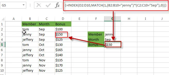
For example, if you want to search for the bonus values that matches the two criteria, the member name is equal to “jenny” and the month value is equal to “Sep”. You can write down the following array formula using INDEX function and MATCH function:

=INDEX(D2:D10,MATCH(1,(B2:B10="jenny")*(C2:C10="Sep"),0))

Let’s see how the above formula works:

=(B2:B10=”jenny”)

The above formula will check each item in the range B2:B10 if it is equal to the string “jenny”, if so, returns TRUE. If not, returns FALSE. The returned result is an array like this:

{FALSE;TRUE;FALSE;FALSE;TRUE;FALSE;FALSE;TRUE;FALSE}

The position of the “TRUE” value in the above array result is actually the position of the lookup value in the range B2:B10.

 

=(C2:C10=”Sep”)

The above formula returns an array result like this:

{TRUE;TRUE;TRUE;FALSE;FALSE;FALSE;FALSE;FALSE;FALSE}

It will check each item in the range C2:C10 if it is equal to the string “Sep”. If so, it returns TRUE, or returns FALSE. From the position of the TRUE value in the array result, you can get the position of the lookup value that matched the criteria in the range C2:C10.

 

=(B2:B10=”jenny”)*(C2:C10=”Sep”)

This formula will convert the TRUE FALSE values to 1s and 0s, and then perform multiplication operation to return the below array result. The position of item “1s” in the array is the position of lookup values matching multiple criteria in the range D2:D10. So you can use the MATCH function to search for 1 value to get the position result.

{0;1;0;0;0;0;0;0;0}

 

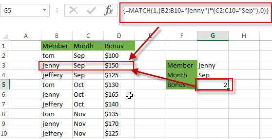
{=MATCH(1,(B2:B10=”jenny”)*(C2:C10=”Sep”),0)}

The MATCH function returns the position number of the lookup bonus value that matching two criteria. It returns 2.

=INDEX(D2:D10,MATCH(1,(B2:B10=”jenny”)*(C2:C10=”Sep”),0))

The INDEX function returns the bonus value at a position returned by the MATCH function. It returns $150.

Using LOOKUP function

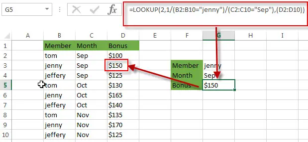
You can also use the LOOKUP function to search for the value with multiple criteria, just refer to the following formula to lookup bonus values that matches two criteria (member name =”jenny” and Month value =”Sep”):

=LOOKUP(2,1/(B2:B10="jenny")/(C2:C10="Sep"),(D2:D10))

Let’s see how this formula works:

=(B2:B10=”jenny”)/(C2:C10=”Sep”)

This formula perform a division operation to get an array result like this:

{0;1;0;#DIV/0!;#DIV/0!;#DIV/0!;#DIV/0!;#DIV/0!;#DIV/0!}

 

=1/(B2:B10=”jenny”)/(C2:C10=”Sep”)

This formula divides 1 by the above array result to get the following new array like this:

{#DIV/0!;1;#DIV/0!;#DIV/0!;#DIV/0!;#DIV/0!;#DIV/0!;#DIV/0!;#DIV/0!}

The position of item 1 in the array is the position of lookup bonus value matching criteria.

 

=LOOKUP(2,1/(B2:B10=”jenny”)/(C2:C10=”Sep”),(D2:D10))

The LOOKUP function looks up 2 in the above array, matches the nearest smaller value (1), and returns the bonus value from the range D2:D10 that is in the same row.

Using SUMPRODUCT function

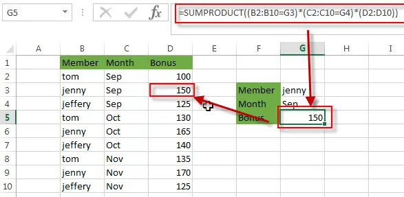
There is another way to search for the value with multiple criteria in excel, using SUMPRODUCT function. You can try to use the following SUMPRODUCT to achieve the same result.

=SUMPRODUCT((B2:B10="jenny")*(C2:C10="Sep")*(D2:D10))

 

Let’s see how this formula works:

=(B2:B10=”jenny”)*(C2:C10=”Sep”)*(D2:D10)

This formula multiples two array results and values in range D2:D10 together and returns another array result like this:

{0;150;0;0;0;0;0;0;0}

 

=SUMPRODUCT((B2:B10=”jenny”)*(C2:C10=”Sep”)*(D2:D10))

The SUMPRODUCT function multiples the items in the arrays and returns sum of the results. So it returns 150.

---

Related Formulas

• Reverse a List or Range
  If you want to reverse a list or range, you can use a combination of the INDEX function, the COUNTA function, the ROW function or ROWS function to create a new formula. you can use the following formula:=INDEX($A$2:$A$5,COUNTA($A$2:$A$5)-ROWS($C$2:C2)+1)…
• Transpose Values Based on the Multiple Lookup Criteria
  If you want to lookup the value with multiple criteria, and then transpose the last results, you can use the INDEX function with the MATCH function to create a new formula.…

Related Functions

• Excel INDEX function
  The Excel INDEX function returns a value from a table based on the index (row number and column number)The INDEX function is a build-in function in Microsoft Excel and it is categorized as a Lookup and Reference Function.The syntax of the INDEX function is as below:= INDEX (array, row_num,[column_num])…
• Excel MATCH function
  The Excel MATCH function search a value in an array and returns the position of that item.The syntax of the MATCH function is as below:= MATCH  (lookup_value, lookup_array, [match_type])….
• Excel LOOKUP function
  The Excel LOOKUP function will search a value in a vector or array.The LOOKUP function is a build-in function in Microsoft Excel and it is categorized as a Lookup and Reference Function.The syntax of the LOOKUP function is as below:= LOOKUP (lookup_value, lookup_vector, [result_vector])….
• Excel SUMPRODUCT function
  The Excel SUMPRODUCT function multiplies corresponding components in the given one or more arrays or ranges, and returns the sum of those products. And it returns a numeric value.The syntax of the SUMPRODUCT function is as below:= SUMPRODUCT (array1,[array2],…)….