This post will guide you how to reverse a list of values or a range of values in excel. How to reverse the order of a column data or a list of items using excel formula. How to reverse a range with sort command. How to reverse a list or column value with VBA.

• Reverse a List or Range with Formula
• Reverse a List or Range with Sort command
• Reverse a List or Range with VBA

Reverse a List or Range with Formula

If you want to reverse a list or range, you can use a combination of the INDEX function, the COUNTA function, the ROW function or ROWS function to create a new formula.

For example, to reverse the range A2:A5, you can use the following formula:

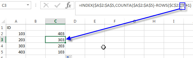
=INDEX($A$2:$A$5,COUNTA($A$2:$A$5)-ROWS($C$2:C2)+1)

Let’s see how the above formulas works:

= COUNTA($A$2:$A$5)

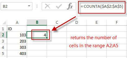
The COUNTA function returns the number of cells in the range A2:A5.  The above COUNTA formula used the absolute reference as its arguments, so it won’t be changed when dragging Fill handle to other single cell.

 

=ROWS($C$2:C2)

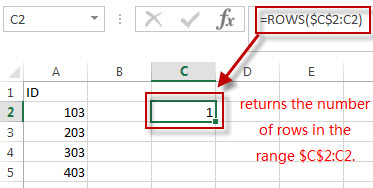
The ROWS function returns the number of rows in the range $C$2:C2. The first Cell is an absolute reference and the second Cell is a relative reference in the argument of the ROWS function. So the second Cell reference can be changed when dragging the Fill handle.

 

= COUNTA($A$2:$A$5)-ROWS($C$2:C2)+1

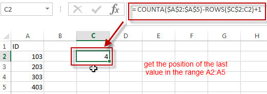
The number of Cells in the range ($A$2:$A$5 subtracted the number of rows in the range $C$2:C2, then add 1, it returns the position of the last value in the range A2:A5. And it returns 4.

 

=INDEX($A$2:$A$5,COUNTA($A$2:$A$5)-ROWS($C$2:C2)+1)

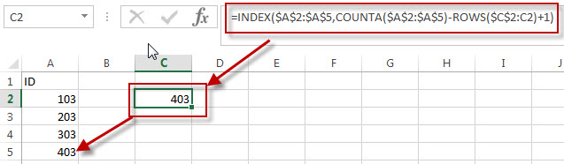
We can use the INDEX function to extract the value based on the position result returned by the above COUNTA-ROWS formula.  So it returns value 403.

Next, we just need to drag the Fill Handler in Cell C1 to other single cells, such as: C2,C3,C4…

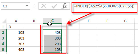
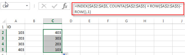
You can also use the below two excel formula to reverse a list or a range:

=INDEX($A$2:$A$5,ROWS(C2:C$5))

=INDEX($A$2:$A$5, COUNTA($A$2:$A$5) + ROW($A$2:$A$5)-ROW(),1)

Reverse a List or Range with Sort command

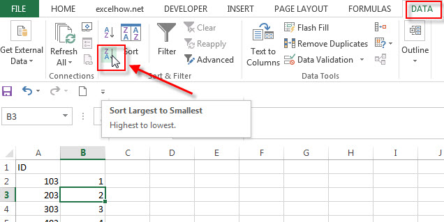
You can also use the Sort command to reverse a list or a range in excel, for example, if you want to reverse the values in the range A2:A5, just refer to the following steps:

1# enter the value 1 into the cell B2, and then fill cells to B5 with a series by using the fill handle.

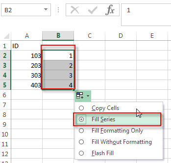
2# click any cell in the range B2:B5

3# click “Sort Z to A”command under Data tab.

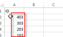
4# delete the Column B, you will see that the range A2:A5 is reversed.

Reverse a List or Range with VBA

You can follow the below steps to create a new excel macro to reverse a list or range in Excel VBA:

1# click on “Visual Basic” command under DEVELOPER Tab.

2# then the “Visual Basic Editor” window will appear.

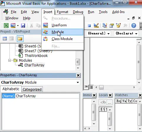
3#click “Insert” ->”Module” to create a new module.

4# paste the below VBA code into the code window. Then clicking “Save” button.

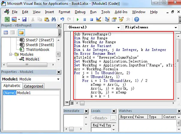
Sub ReverseRange()
    Dim Rng As Range
    Dim WorkRng As Range
    Dim Arr As Variant
    Dim i As Integer, j As Integer, k As Integer
    On Error Resume Next
    xTitleId = "ReverseColumnValue"
    Set WorkRng = Application.Selection
    Set WorkRng = Application.InputBox("Range", xTitleId, WorkRng.Address, Type:=8)
    Arr = WorkRng.Formula
    For j = 1 To UBound(Arr, 2)
        k = UBound(Arr, 1)
        For i = 1 To UBound(Arr, 1) / 2
            xTemp = Arr(i, j)
            Arr(i, j) = Arr(k, j)
            Arr(k, j) = xTemp
            k = k - 1
        Next
    Next
    WorkRng.Formula = Arr
End Sub

5# back to the current workbook, then click Macros button under DEVELOPER tab, or Press F5 key to run the above macro.

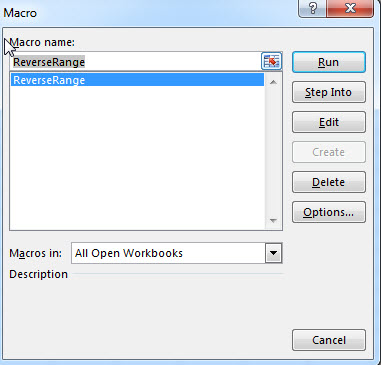
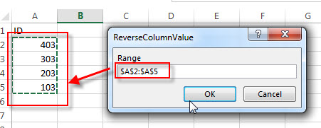
6# click “RUN” button, then input the range value A2:A5 that you want to reverse.

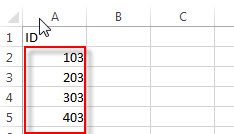
7# let’s see that last result.

---

Related Formulas

• Find the Relative Position in a Range or Table
  If you want to know the relative row position for all rows in an Excel Range (B3:D6), you can use a excel Array formula as follows:=ROW(B3:D6)- ROW(B3) + 1. You can also use another excel array formula to get the same result as follows:=ROW(B3:D6)-ROW(INDEX(B3:D6,1,1))+1…
• Lookup the Next Largest Value
  If you want to get the next largest value in another column, you can use a combination of the INDEX function and the MATCH function to create an excel formula.you can use the following formula:=INDEX(A2:A5,MATCH(200,A2:A5)+1)…

Related Functions

• Excel INDEX function
  The Excel INDEX function returns a value from a table based on the index (row number and column number)The INDEX function is a build-in function in Microsoft Excel and it is categorized as a Lookup and Reference Function.The syntax of the INDEX function is as below:= INDEX (array, row_num,[column_num])…
• Excel ROW function
  The Excel ROW function returns the row number of a cell reference.The ROW function is a build-in function in Microsoft Excel and it is categorized as a Lookup and Reference Function.The syntax of the ROW function is as below:= ROW ([reference])….
• Excel COUNTA function
  The Excel COUNTA function counts the number of cells that are not empty in a range. And it returns the number of non-blank cells within a range or value. The syntax of the COUNTA function is as below:= COUNTA(value1, [value2],…)
• Excel ROWS function
  The Excel ROWS function returns the number of rows in a cell reference.The ROWS function is a build-in function in Microsoft Excel and it is categorized as a Lookup and Reference Function.The syntax of the ROWS function is as below:= ROWS(array)…