This post explains that how to get the unique values from a range or column in excel. How to extract unique values from a list or excel range in excel 2013.

Extract unique values

If you want to extract a list of unique items from a column or range, you can use a combination of the IFERROR function, the INDEX function, the MATCH function and the COUNTIF function to create an array formula.

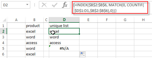
For example, to extract unique values from the range B2:B6, then display the unique values in column D, you can use the following array formula:

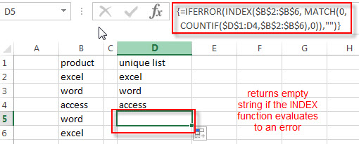
=IFERROR(INDEX($B$2:$B$6, MATCH(0, COUNTIF($D$1:D1,$B$2:$B$6),0)),"")

Note: when you enter the above array formula, you must hold the Control and Shift keys down, then press Enter. Then the formula bar should add curly braces surrounding the array formula.

Let’s see how this formula works:

= COUNTIF($D$1:D1,$B$2:$B$6)

The COUNTIF function counts the number of the unique values in the unique list (column D) appear in the range B2:B6. And the first range starts in the absolute reference of Cell D1. And the above formula need to enter in the Cell D2.  It returns an array like this:

{0;0;0;0;0}

When you drag the Fill Handle down to other cells, such as: D3, D4…. This formula return the following array result:

{1;0;0;0;1}

{1;1;0;1;0}

= MATCH(0, COUNTIF($D$1:D1,$B$2:$B$6),0))

The MATCH function returns the position of the first lookup value “0” in the array result returned by the COUNTIF function. The position number goes into the INDEX function as its row_num argument.

 

=INDEX($B$2:$B$6, MATCH(0, COUNTIF($D$1:D1,$B$2:$B$6),0))

The INDEX function extracts the value from range B2:B6 based on the position returned by the MATCH function. So it returns the first unique value in range B2:B6.

If you need to get the second or nth unique values in range B2:B6, then you just need to drag the Fill Handle to other cells.

 

=IFERROR()

If the INDEX function returns a #N/A error, and the IFERROR function will capture this excel error (#N/A!), then returns an alternate value.

---

Related Formulas

• Get the First Match in Two Excel Ranges
  If you want to find the first match between two excel ranges, you can use a combination of the INDEX function, the MATCH function and COUNTIF function to create a new formula….
• Get Cell Address of a Lookup Value
  If you want to lookup a value in a range or column and return the cell address of the first match of lookup value, you can use a combination with the CELL function, the INDEX function and the MATCH function…
• Find the nth Smallest Value
  You can use the SMALL function to get the 1st, 2nd, 3rd, or nth smallest value in an array or range. Also you can use the SMALL function within the INDEX function to extract the relative value of the same row…

Related Functions

• Excel IFERROR function
  The Excel IFERROR function returns an alternate value you specify if a formula results in an error, or returns the result of the formula.The syntax of the IFERROR function is as below:= IFERROR (value, value_if_error)…
• Excel COUNTIF function
  The Excel COUNTIF function will count the number of cells in a range that meet a given criteria. This function can be used to count the different kinds of cells with number, date, text values, blank, non-blanks, or containing specific characters.etc.= COUNTIF (range, criteria)…
• Excel INDEX function
  The Excel INDEX function returns a value from a table based on the index (row number and column number)The INDEX function is a build-in function in Microsoft Excel and it is categorized as a Lookup and Reference Function.The syntax of the INDEX function is as below:= INDEX (array, row_num,[column_num])…
• Excel MATCH function
  The Excel MATCH function search a value in an array and returns the position of that item.The syntax of the MATCH function is as below:= MATCH  (lookup_value, lookup_array, [match_type])….