This post explains that how to transpose values from columns to rows based on the multiple lookup criteria in excel.

In the previous, we talked that how to transpose values from columns to rows using Paste Special Transpose, it’s just rearrange all data in a range and do not apply for any criteria.

1. Transpose Values Based on the Multiple Lookup Criteria

If you want to lookup the value with multiple criteria, and then transpose the last results, you can use the INDEX function with the MATCH function to create a new formula.

For example, to transpose the values in both column B and Column C based on the multiple criteria: member’s name is equal to the range B2:B10, and month’s value is equal to the range C2:C10, then extract the bonus value from the range D2:D10. you can use the following array formula:

=INDEX($D$2:$D$10,MATCH(1,($B$2:$B$10=$F4)*($C$2:$C$10=G$3),0))

Let’s see how the above formula works:

=($B$2:$B$10=$F4)

The above formula will check if each value in the range B2:B10 is equal to the value in Cell F4, if so, return TRUE, otherwise, returns FALSE. So the above formula returns an array result like this:

{TRUE;FALSE;FALSE;TRUE;FALSE;FALSE;TRUE;FALSE;FALSE}

=($C$2:$C$10=G$3)

The above formula will check if each month value in the range C2:C10 is equal to the value in Cell G3, if so, return TRUE, otherwise, returns FALSE. So the above formula returns an array result like this:

{TRUE;TRUE;TRUE;FALSE;FALSE;FALSE;FALSE;FALSE;FALSE}

=($B$2:$B$10=$F4)*($C$2:$C$10=G$3)

the above formula returns an array result like this:

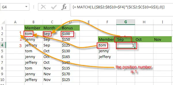
{1;0;0;0;0;0;0;0;0}

= MATCH(1,($B$2:$B$10=$F4)*($C$2:$C$10=G$3),0)

The MATCH function used the above array result(containing one and zero) to find the position of item “1”, it is actually the position of the bonus value that matched the multiple criteria.

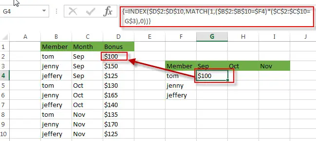
=INDEX($D$2:$D$10,MATCH(1,($B$2:$B$10=$F4)*($C$2:$C$10=G$3),0))

The INDEX function extracts the value based on the position result returned by the above MATCH function. So it returns “$100”in Cell G4.

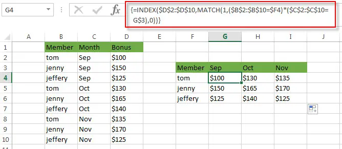
You can drag the Fill Handler in the Cell G4 to other cells to fill up the entire range G4:I6 as you need.

2. Video: Transpose Values Based on the Multiple Lookup Criteria in Excel

This video will show you how to use an array formula to transpose values based on multiple lookup criteria in Excel.

3. Related Formulas

• Reverse a List or Range
  If you want to reverse a list or range, you can use a combination of the INDEX function, the COUNTA function, the ROW function or ROWS function to create a new formula. you can use the following formula:=INDEX($A$2:$A$5,COUNTA($A$2:$A$5)-ROWS($C$2:C2)+1)…
• Lookup the Value with Multiple Criteria
  If you want to lookup the value with multiple criteria in a range, you can use a combination with the INDEX function and MATCH function to create an array formula…

4. Related Functions

• Excel INDEX function
  The Excel INDEX function returns a value from a table based on the index (row number and column number)The INDEX function is a build-in function in Microsoft Excel and it is categorized as a Lookup and Reference Function.The syntax of the INDEX function is as below:= INDEX (array, row_num,[column_num])…
• Excel MATCH function
  The Excel MATCH function search a value in an array and returns the position of that item.The syntax of the MATCH function is as below:= MATCH  (lookup_value, lookup_array, [match_type])….