This post explains that how to use two way lookup formula to find a value in a table or in a two dimensional range in excel. How to lookup a value in a table using given row and column with INDEX and MATCH functions. Or how to do perform a two way lookup with VLOOKUP function.

As the lookup functions in excel are only support to perform one-way lookups, so there is no built-in function to do a two-way lookup, the below will talk that how to create a new excel formula to perform two-way lookup in excel.

• Two way lookup with index/match
• Two way lookup with VLOOKUP

 

Two way lookup with index/match

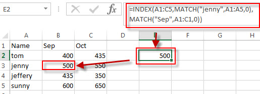
If you want to look up a value in a table using both rows and columns, you can use a combination with the INDEX function and the MATCH function to create an excel formula. For example, if you have a salary table and you want to find jenny’s salary in Sep in the two dimensional range A1:C5, you can write down the following two-way lookup formula with INDEX function and MATCH function:

=INDEX(A1:C5,MATCH("jenny",A1:A5,0),MATCH("Sep",A1:C1,0))

Let’s see how this formula works:

The MATCH function returns the relative position of a lookup value in the range A1:A5 or A1:C1. And the match_type is set to 0, it means that the MATCH function lookup the first match of the value that is exactly equal to the lookup value.

= MATCH(“jenny”,A1:A5,0)

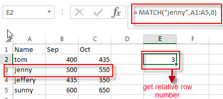
So the first MATCH function returns the first position of string “jenny” in the range A1:A5. It returns 3. It will goes into the INDEX function as its row_num argument.

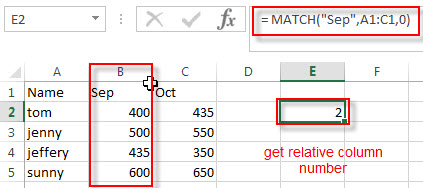
= MATCH(“Sep”,A1:C1,0)

 

And the second MATCH function will return the position of the first occurrence of the string “Sep” in the range A1:C1. It returns 2 and it will goes into the INDEX function as its column_num argument.

So we can get the row number as 3 and the column number is 2 from the MATCH function.

 

=INDEX(A1:C5,3,2)

The INDEX function returns the value at the intersection of row 3 and column 2 in the range A1:C5.

Two way lookup with VLOOKUP

You can also use the VLOOKUP function to build an excel formula to perform a two-way lookup in excel. You can try to use the following formula:

=VLOOKUP("jenny",A1:C5,MATCH("Sep",A1:C1,0),FALSE)

Let’s see how this formula works:

=MATCH(“Sep”,A1:C1,0)

As I said above, the MATCH function returns the relative position of the first occurrence of the string “Sep” in the range A1:C1. It returns 2. This value will go into the VLOOKUP function as its column_index_num argument.

 

=VLOOKUP(“jenny”,A1:C5,MATCH(“Sep”,A1:C1,0),FALSE)

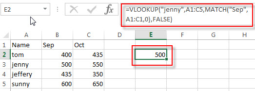
The VLOOKUP function lookup string “jenny” in the first column of the range A1:C5 and then returns the value in the same row based on the column_index_num value returned by the above MATCH function.

---

Related Formulas

• Lookup Entire Row using INDEX/MATCH
  If you want to lookup entire row and then return all values of the matched row, you can use a combination of the INDEX function and the MATCH function to create a new excel array formula.
• Extract the Entire Column of a Matched Value
  If you want to lookup value in a range and then retrieve the entire row, you can use a combination of the INDEX function and the MATCH function to create a new excel formula..…
• Lookup the Next Largest Value
  If you want to get the next largest value in another column, you can use a combination of the INDEX function and the MATCH function to create an excel formula..

Related Functions

• Excel VLOOKUP function
  The Excel VLOOKUP function lookup a value in the first column of the table and return the value in the same row based on index_num position.The syntax of the VLOOKUP function is as below:= VLOOKUP (lookup_value, table_array, column_index_num,[range_lookup])…
• Excel INDEX function
  The Excel INDEX function returns a value from a table based on the index (row number and column number)The INDEX function is a build-in function in Microsoft Excel and it is categorized as a Lookup and Reference Function.The syntax of the INDEX function is as below:= INDEX (array, row_num,[column_num])…
• Excel MATCH function
  The Excel MATCH function search a value in an array and returns the position of that item.The syntax of the MATCH function is as below:= MATCH  (lookup_value, lookup_array, [match_type])….