This post explains that how to get the nth occurrence value with multiple criteria using INDEX and MATCH in excel. How to find the first, second or nth match with multiple criteria in excel. How to return the nth match on a multiple criteria using INDEX and MATCH.

In the previous post, we talked that get the nth match value with only one criteria.

Also, we also talked that how to Lookup the Value with Multiple Criteria to find the first occurrence match in excel.

1. Find nth Occurrence with Multiple Criteria Using Formula

If you want to find the nth occurrence with multiple criteria, you can use a combination with the INDEX function, SMALL function, nested IF function and ROW function to create a complex excel formula like this:

=INDEX(Array,SMALL(IF(Range1=Criteria1,IF(Range2=Criteria2,IF(Range3=Criteria3,IF(Range4=Criteria4,IF(Range5=Criteria5,ROW(Array)-ROW(INDEX(Array,1))+1))))),nth))

For example, if you want to get the bonus value in the excel range D2:D10 that must meet two criteria, and the first one is that the member name is equal to the string “jenny” in the range A2:A10, and the second criteria is that the location is equal to “London” in the range B2:B10. So we can write down the following array formula:

=INDEX(D2:D10, SMALL(IF(A2:A10="jenny",IF(B2:B10="London", ROW(A2:A10)-ROW(INDEX(A2:A10,1,1))+1)),2))

Note: after entering this formula in the formula bar, you need to press CTRL+SHIFT+Enter key to convert it as array formula.

Let’s see how this formula works:

=ROW(A2:A10)-ROW(INDEX(A2:A10,1,1))+1

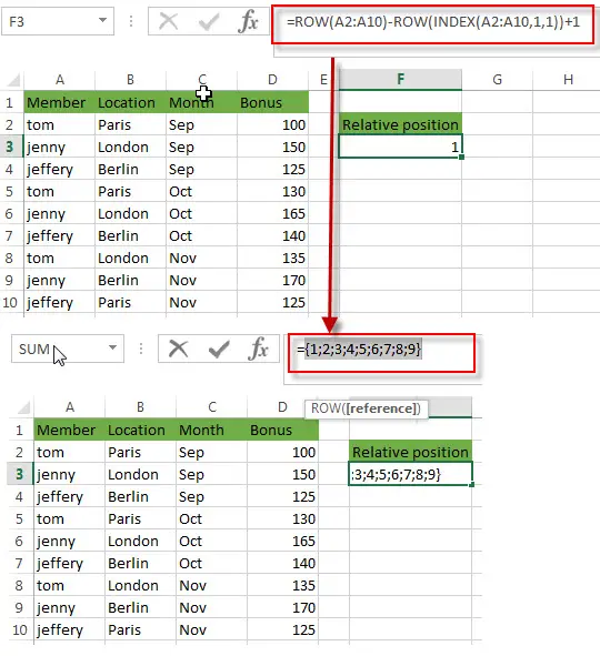
This formula returns the relative position of the range A2:A10, it returns an array result like this:

{1;2;3;4;5;6;7;8;9}

For More detailed description, you can continue to read this post: How to Find the Relative Position in a Range or Table

=IF(A2:A10=”jenny”,IF(B2:B10=”London”, ROW(A2:A10)-ROW(INDEX(A2:A10,1,1))+1))

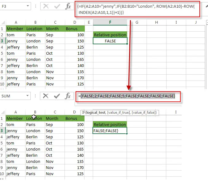
This function is a nested IF function, it will check each item of range A2:A10 firstly and if it is equal to the string “jenny”, if TRUE, then continue to check each item of range B2:B10 if it is equal to the string “London”, if TRUE, return the relative position of row. Otherwise, return FALSE. So this formula returns an array result like this:

{FALSE;2;FALSE;FALSE;5;FALSE;FALSE;FALSE;FALSE}

=SMALL(IF(A2:A10=”jenny”,IF(B2:B10=”London”, ROW(A2:A10)-ROW(INDEX(A2:A10,1,1))+1)),2)

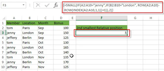
The SMALL function returns the second smallest value from the array result returned by the above nested IF function. It returns 5.

So far, we got the position of the second occurrence of bonus value that meet two criteria as requested above.

=INDEX(D2:D10, SMALL(IF(A2:A10=”jenny”,IF(B2:B10=”London”, ROW(A2:A10)-ROW(INDEX(A2:A10,1,1))+1)),2))

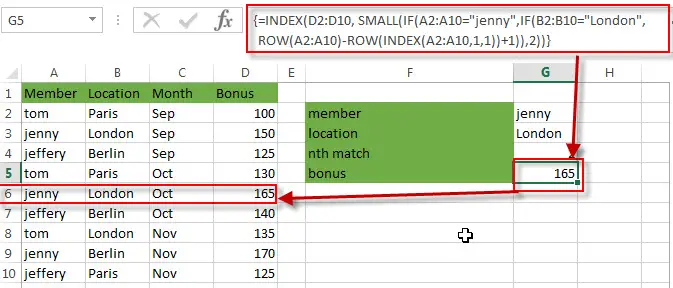
The INDEX function extract the values at a position that returned by the SMALL function. So it is the bonus value of the second occurrence in the range D2:D10. It is 165.

2. Find nth Occurrence with Multiple Criteria Using VBA Code

Now, moving on to the second method, we’ll explore the power of VBA code to achieve the same task. This method offers additional customization options and automation capabilities, making it suitable for more complex scenarios or repetitive tasks.

Press ‘Alt + F11’ to open the Visual Basic for Applications  editor.

Right-click on any item in the project explorer , hover over “Insert” and select “Module” to add a new module.

In the newly created module, copy and paste the following VBA code:

Function FindNthOccurrence(criteria1 As Range, criteria2 As Range, nth As Integer, dataRange As Range)
    Dim i As Long
    Dim count As Long
    
    count = 0
    
    For i = 1 To dataRange.Rows.count
        If dataRange.Cells(i, 1).Value = criteria1.Value And dataRange.Cells(i, 2).Value = criteria2.Value Then
            count = count + 1
            If count = nth Then
                FindNthOccurrence = dataRange.Cells(i, 3).Value
                Exit Function
            End If
        End If
    Next i
    
    FindNthOccurrence = "Not Found"
End Function

Close the VBA editor by clicking the “X” button or pressing ‘Alt + Q’. Return to your Excel workbook.

In any cell where you want to display the result, enter the formula like this:

=FindNthOccurrence(F2, F3, F4, A2:C10)

Replace “criteria1” and “criteria2” with the criteria you’re searching for, “nth” with the occurrence number you’re looking for, and “dataRange” with the range where you’re searching.

After entering the formula, press Enter to execute it.

The VBA function will search for the nth occurrence that matches the specified criteria in the given range and display the result.

3. Video: Find nth Occurrence with Multiple Criteria

This Excel video tutorial where we’ll explore two methods to find the nth occurrence with multiple criteria. We delve into the first method using a formula based on the INDEX and MATCH functions, followed by the second method utilizing VBA code.

https://youtu.be/0lxI2hiLLxk

4. Related Formulas

• Get nth Match with One Criteria using INDEX/MATCH
  if you want to find the 2th occurrence of the member “jenny” in the range B2:B10 and extracts its relative bonus value in the range D2:D10, you can used the following array formula:=INDEX(D2:D10, SMALL(IF(B2:B10=”jenny”, ROW(B2:B10)-ROW(INDEX(B2:B10,1,1))+1),2))…
• Reverse a List or Range
  If you want to reverse a list or range, you can use a combination of the INDEX function, the COUNTA function, the ROW function or ROWS function to create a new formula. you can use the following formula:=INDEX($A$2:$A$5,COUNTA($A$2:$A$5)-ROWS($C$2:C2)+1)…
• Transpose Values Based on the Multiple Lookup Criteria
  If you want to lookup the value with multiple criteria, and then transpose the last results, you can use the INDEX function with the MATCH function to create a new formula.…
• Lookup the Value with Multiple Criteria
  If you want to lookup the value with multiple criteria in a range, you can use a combination with the INDEX function and MATCH function to create an array formula.…
• Lookup the Next Largest Value
  If you want to get the next largest value in another column, you can use a combination of the INDEX function and the MATCH function to create an excel formula..

5. Related Functions

• Excel INDEX function
  The Excel INDEX function returns a value from a table based on the index (row number and column number)The INDEX function is a build-in function in Microsoft Excel and it is categorized as a Lookup and Reference Function.The syntax of the INDEX function is as below:= INDEX (array, row_num,[column_num])…
• Excel MATCH function
  The Excel MATCH function search a value in an array and returns the position of that item.The syntax of the MATCH function is as below:= MATCH  (lookup_value, lookup_array, [match_type])….
• Excel SMALL function
  The Excel SMALL function returns the smallest numeric value from the numbers that you provided. Or returns the smallest value in the array.The syntax of the SMALL function is as below:=SMALL(array,nth) …
• Excel ROW function
  The Excel ROW function returns the row number of a cell reference.The ROW function is a build-in function in Microsoft Excel and it is categorized as a Lookup and Reference Function.The syntax of the ROW function is as below:= ROW ([reference])….
• Excel nested IF function
  The nested IF function is formed by multiple if statements within one Excel if function. This excel nested if statement makes it possible for a single formula to take multiple actions.The syntax of Nested IF function is as below:=IF(Condition_1,Value_if_True_1,IF(Condition_2,Value_if_True_2,Value_if_False_2))….
• Excel IF function
  The Excel IF function perform a logical test to return one value if the condition is TRUE and return another value if the condition is FALSE. The IF function is a build-in function in Microsoft Excel and it is categorized as a Logical Function.The syntax of the IF function is as below:= IF (condition, [true_value], [false_value])….