This post will guide you how to transpose multiple columns into a single columns with multiple rows in Excel. How do I put data from multiple columns into one column with Excel formula; How to transpose columns into single column with VBA macro in excel.

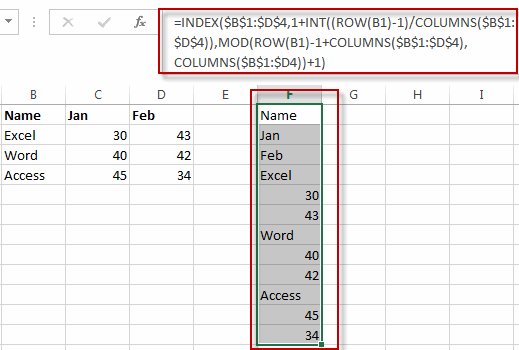
Assuming that you have a data list in range B1:D4 contain 3 columns and you want to transpose them into a single column F. just following the below two ways.

1. Transpose Multiple Columns into One Column with Formula

You can use the following excel formula to transpose multiple columns that contain a range of data into a single column F:

#1 type the following formula in the formula box of cell F1, then press enter key.

=INDEX($B$1:$D$4,1+INT((ROW(B1)-1)/COLUMNS($B$1:$D$4)),MOD(ROW(B1)-1+COLUMNS($B$1:$D$4),COLUMNS($B$1:$D4))+1)

#2 select cell F1, then drag the Auto Fill Handler over other cells until all values in range B1:D4 are displayed.

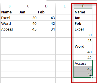
#3 you will see that all the data in range B1:D4 has been transposed into single column F.

2. Transpose Multiple Columns into One Column with VBA Macro

You can also write an Excel VBA Macro to transpose the data of range in B1:D4 into single column F quickly. Just do the following steps:

#1 click on “Visual Basic” command under DEVELOPER Tab.

#2 then the “Visual Basic Editor” window will appear.

#3 click “Insert” ->”Module” to create a new module.

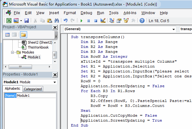
#4 paste the below VBA code into the code window. Then clicking “Save” button.

Sub transposeColumns()
    Dim R1 As Range
    Dim R2 As Range
    Dim R3 As Range
    Dim RowN As Integer
    wTitle = "transpose multiple Columns"
    Set R1 = Application.Selection
    Set R1 = Application.InputBox("please select the Source data of Ranges:", wTitle, R1.Address, Type:=8)
    Set R2 = Application.InputBox("Select one destination single Cell or column:", wTitle, Type:=8)
    RowN = 0
    Application.ScreenUpdating = False
    For Each R3 In R1.Rows
        R3.Copy
        R2.Offset(RowN, 0).PasteSpecial Paste:=xlPasteAll, Transpose:=True
        RowN = RowN + R3.Columns.Count
    Next
    Application.CutCopyMode = False
    Application.ScreenUpdating = True
End Sub

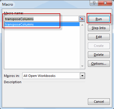
#5 back to the current worksheet, then run the above excel macro. Click Run button.

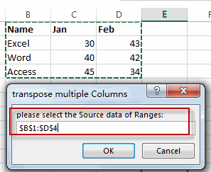
#6 select the source data of ranges, such as: B1:D4

#7 select one single cell in the destination Column, such as: F1

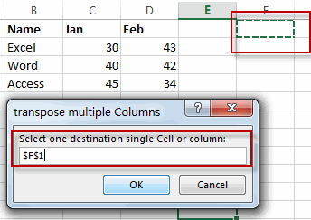
#8 let’s see the last result.

3. Video: Transpose Multiple Columns into One Column

This video tutorial, we’ll tackle the task of transposing multiple columns into a single column throught two approaches: using a formula and creating a VBA macro in Excel.

https://youtu.be/xRID6DewKOE

4. Related Functions

• Excel INDEX function
  The Excel INDEX function returns a value from a table based on the index (row number and column number)The INDEX function is a build-in function in Microsoft Excel and it is categorized as a Lookup and Reference Function.The syntax of the INDEX function is as below:= INDEX (array, row_num,[column_num])…
• Excel INT function
  The Excel INT function returns the integer portion of a given number. And it will rounds a given number down to the nearest integer.  And the INT function rounds down, so if you provide a negative number, the returned value will become more negative.The syntax of the INT function is as below:= INT (number)…
• Excel ROW function
  The Excel ROW function returns the row number of a cell reference.The ROW function is a build-in function in Microsoft Excel and it is categorized as a Lookup and Reference Function.The syntax of the ROW function is as below:= ROW ([reference])….
• Excel Columns function
  The Excel COLUMNS function returns the number of columns in an Array or a reference.The syntax of the COLUMNS function is as below:=COLUMNS (array)….
• Excel MOD function
  he Excel MOD function returns the remainder of two numbers after division. So you can use the MOD function to get the remainder after a number is divided by a divisor in Excel. The syntax of the MOD function is as below:=MOD (number, divisor)….