In the previous post, we talked that how to get the nth smallest value in a range and how to get the relative value of the same row of the nth smallest value in a range or array. And this post will guide you how to get the nth largest value in a range in excel. How to extract the relative value based on the position of the nth largest value in a single column.

Find the nth Largest Value

To get the 1st, 2nd, 3rd, or nth largest value in a range (single column, or row), you can use the LARGE function.

For example:

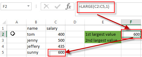
Find the First Largest Value

You can use the following formula to get the first largest value in the range C2:C5:

=LARGE(C2:C5,1)

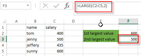
Find the Second Largest Value

To get the second largest value in the range C2:C5, you can use the following LARGE function:

=LARGE(C2:C5,2)

Find the nth Largest Value

you just need to modify the second argument (nth) of the LARGE function to a numeric value that you want. Refer to the below formula:

=LARGE(C2:C5,nth)

 

Get the Relative value

If you want to get the relative value of the same row of the nth largest value, you can use a combination with the LARGE function, the INDEX function and MATCH function. For example, to get the name value in the same relative row position of the second largest salary value in the range C2:C5, you can use the following excel formula:

=INDEX(B2:B5,MATCH(LARGE(C2:C5,2),C2:C5,0))

 

Let’s see how this formula works:

=LARGE(C2:C5,2)

As described above, This LARGE function returns the second largest value in the range C2:C5.

 

=MATCH(LARGE(C2:C5,2),C2:C5,0)

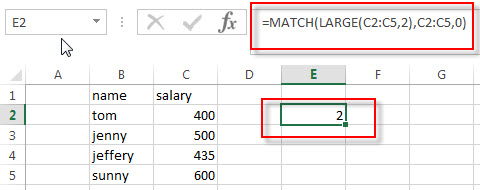
The MATCH function will perform an exact searching in the range C2:C5, then returns the position number of the second largest value in the range C2:C5. It returns 2.

 

=INDEX(B2:B5,MATCH(LARGE(C2:C5,2),C2:C5,0))

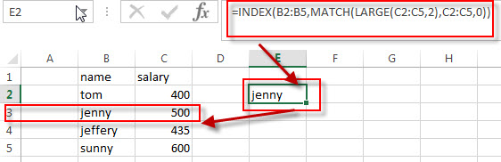
The INDEX function extract the value based on the position number that returned by the above MATCH function, so it returns one value in the range B2:B5 based on the returned position. It returns “jenny”.

---

Related Formulas

• Get nth Match with One Criteria using INDEX/MATCH
  if you want to find the 2th occurrence of the member “jenny” in the range B2:B10 and extracts its relative bonus value in the range D2:D10, you can used the following array formula:=INDEX(D2:D10, SMALL(IF(B2:B10=”jenny”, ROW(B2:B10)-ROW(INDEX(B2:B10,1,1))+1),2))…
• Lookup the Value with Multiple Criteria
  If you want to lookup the value with multiple criteria in a range, you can use a combination with the INDEX function and MATCH function to create an array formula.…
• Lookup the Next Largest Value
  If you want to get the next largest value in another column, you can use a combination of the INDEX function and the MATCH function to create an excel formula..
• Find the nth Smallest Value
  You can use the SMALL function to get the 1st, 2nd, 3rd, or nth smallest value in an array or range. Also you can use the SMALL function within the INDEX function to extract the relative value of the same row…

Related Functions

• Excel INDEX function
  The Excel INDEX function returns a value from a table based on the index (row number and column number)The INDEX function is a build-in function in Microsoft Excel and it is categorized as a Lookup and Reference Function.The syntax of the INDEX function is as below:= INDEX (array, row_num,[column_num])…
• Excel MATCH function
  The Excel MATCH function search a value in an array and returns the position of that item.The syntax of the MATCH function is as below:= MATCH  (lookup_value, lookup_array, [match_type])….
• Excel LARGE function
  The Excel LARGE function returns the largest numeric value from the numbers that you provided. Or returns the largest value in the array. The syntax of the LARGE function is as below:= LARGE (array,nth)…