How to get the relative row numbers for a range or table. How to find the relative row position of one Cell value in a specified Range or table. This post will guide you how to get the relative position of all rows in a range or table in excel. And how to get the relative row position of an item in a table or excel range.

• Get the Relative Row Position of all Rows in Range
• Get the Relative Row number of an item in a Range

Get the Relative Row Position of all Rows in Range

Supposing that you have a table that contain the data as the below picture.

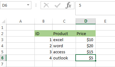
If you want to know the relative row position for all rows in an Excel Range (B3:D6), you can use a excel Array formula as follows:

=ROW(B3:D6)- ROW(B3) + 1

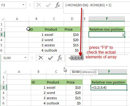
Note: when you enter into the above formula in Cell F3, you must be press “CTRL”+”Shift”+ Enter to indicate that formula is an array formula.

Let’s see how the above array formula works:

=ROW (B3:D6)

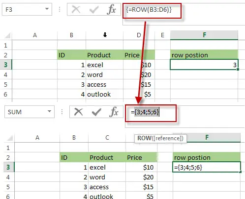
The first ROW function will return an array that contain 4 row numbers (absolute position) as elements.

 

=ROW (B3)

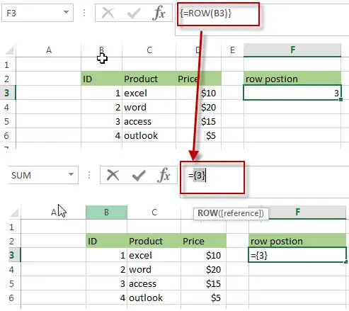
The above Row function in array formula will also return an array contain only one element (row number of Cell B3)

 

=ROW(B3:D6)- ROW(B3)

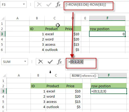
The result returned by the second ROW function is subtracted by the result returned by the First ROW function and it will return another Array as below:

{0;1;2;3}

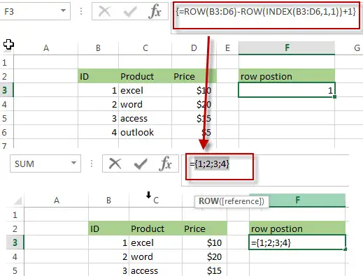
Then the each value in the above array add 1 to get the relative row position of all rows in Range B3:D6, like the below array:

{1;2;3;4}

You can also use another excel array formula to get the same result as follows:

=ROW(B3:D6)-ROW(INDEX(B3:D6,1,1))+1

The INDEX function will return the reference of the first row in the range B3:D6, in other words, returns the reference of Cell B3.

Get the Relative Row number of an item in a Range

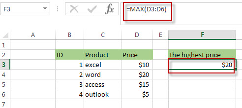
Suppose that you have a table of data such as the above picture. If you want to get the row position of the highest price in a range (B3:D6), you can use the MAX function within the MATCH function to get the relative row position of the highest price in a range or a table. Just using the following excel formula:

=MATCH(MAX(D3:D6),D3:D6,0)

The MAX function returns the highest price as $20 in range D3:D6.

Then the MATCH function will search for a value returned by the MAX function in range D3:D6, then it returns the relative position of $20.

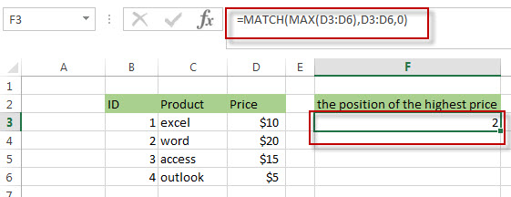
You will see that the above formula returns 2, because the second row in the range of D3:D6 have the highest price.

---

Related Formulas

• Combine Text from Two or More Cells into One Cell
  If you want to combine text from multiple cells into one cell and you can use the Ampersand (&) symbol.If you are using the excel 2016, then you can use a new function TEXTJOIN function to combine text from multiple cells…
• Split Text String to an Array
  If you want to convert a text string into an array that split each character in text as an element, you can use an excel formula to achieve this result. the below will guide you how to use a combination of the MID function, the ROW function, the INDIRECT function and the LEN function to split a string…

Related Functions

• Excel INDEX function
  The Excel INDEX function returns a value from a table based on the index (row number and column number)The INDEX function is a build-in function in Microsoft Excel and it is categorized as a Lookup and Reference Function.The syntax of the INDEX function is as below:= INDEX (array, row_num,[column_num])…
• Excel ROW function
  The Excel ROW function returns the row number of a cell reference.The ROW function is a build-in function in Microsoft Excel and it is categorized as a Lookup and Reference Function.The syntax of the ROW function is as below:= ROW ([reference])….
• Excel MATCH  function
  The Excel MATCH function search a value in an array and returns the position of that item.The MATCH function is a build-in function in Microsoft Excel and it is categorized as a Lookup and Reference Function.The syntax of the MATCH function is as below:= MATCH  (lookup_value, lookup_array, [match_type])….