This post explains that how to extract multiple match values from a range, then put the values into the different columns in excel. And how to extract multiple matches into the different rows.
In the previous post, we talked that how to get the position of the nth occurrence of a value in a column, and this pose will refer to it to extract all matched values firstly, then put all returned values into the different columns.
Table of Contents
1. Extract multiple match values into separate columns
If you want to fetch all matches from a range then put it into cells in different columns, you can use a combination with the INDEX function, the SMALL function, the IF function, the ROW function and the COLUMNS function to create a new excel formula.
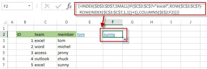
For example, if you want to get all member names belong to “excel” team in the range B3:D7, then separate it into the different columns, such as: E2, F2…you can use the following formula:
=IFERROR(INDEX($D$3:$D$7,SMALL(IF($C$3:$C$7="excel",ROW($C$3:$C$7)-ROW(INDEX($C$3:$C$7,1,1))+1),COLUMNS($E$2:E2))),"")Let’s see how the above formula works:
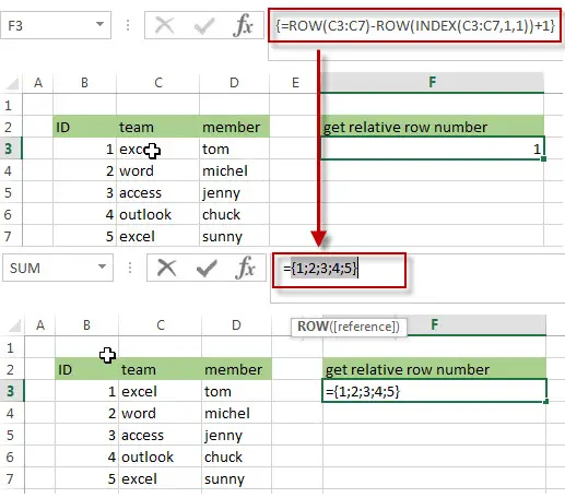
= ROW($C$3:$C$7)-ROW(INDEX($C$3:$C$7,1,1))+1
The ROW function returns the relative position of all rows in the range C3:C7. The returned result is another array.
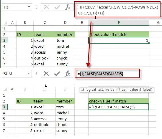
= IF($C$3:$C$7=”excel”,ROW($C$3:$C$7)-ROW(INDEX($C$3:$C$7,1,1))+1)
The IF function will check if each value in range C3:C7 is equal to “excel”, if TRUE, returns its relative position, otherwise, returns FALSE. As this formula is an array formula, so it must be returned an array result.
=COLUMNS($E$2:E2)
The COLUMNS function returns a numeric values, it will be used by the SMALL function as its nth argument to indicate the position of the number that you want to return.
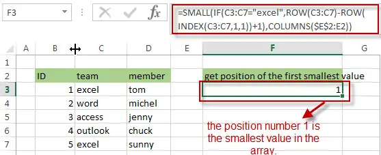
=SMALL(IF($C$3:$C$7=”excel”,ROW($C$3:$C$7)-ROW(INDEX($C$3:$C$7,1,1))+1),COLUMNS($E$2:E2))
The SMALL function returns the position of the nth smallest values from the numbers in an array result returned by the above IF function. The nth argument is specified by the result returned by the COLUMNS function.
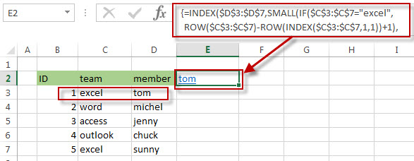
=INDEX($D$3:$D$7,SMALL(IF($C$3:$C$7=”excel”,ROW($C$3:$C$7)-ROW(INDEX($C$3:$C$7,1,1))+1),COLUMNS($E$2:E2)))
The INDEX function returns a value at a position returned by the above SMALL function in the range D3:D7, so it should be the first matches of the member name that belong to the excel team in the range B3:D7.
And if you want to get the second matches into Cell F2, you just need to drag the fill hander in the Cell E2 to F2, then the second matches of the member name will be fetched in the Cell F2.
=IFERROR()
The IFERROR function will check if the result returned by the SMALL function is a #NUM error, then returns an empty string.
2. Extract multiple match values into separate rows
If you want to extract multiple matches into the separate rows in excel, just need to use ROWS instead of the COLUMNS function in the above formula as follows:
=IFERROR(INDEX($D$3:$D$7,SMALL(IF($C$3:$C$7="excel",ROW($C$3:$C$7)-ROW(INDEX($C$3:$C$7,1,1))+1), ROWS($E$2:E2))),"")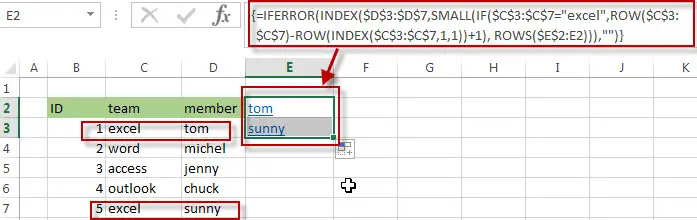
If you want to extract the second matches, then put the result into the cell E3, you just need to drag the Fill Handler in Cell E2 to E3. The second matches of the member name should be fetched in the Cell E3.
3. Extract multiple match Values into different Rows Using User-Defined Function
Let’s delve into how to incorporate this User-Defined Function into your Excel workflow.
Step1: Press Alt + F11 to open the Visual Basic for Applications (VBA) editor.
Step2: Insert a new module and paste the provided VBA code. In the VBA editor, right-click on any item in the project explorer on the left. Choose “Insert” and then “Module” to add a new module.
Step3: Copy the provided VBA code. Paste the code into the code window of the newly created module.
Function ExtractMatches(searchValue As Variant, criteriaRange As Range, dataRange As Range) As Variant
    Dim resultArr() As Variant
    Dim i As Long
    Dim matchCount As Long
    Dim cell As Range

    ' Initialize matchCount
    matchCount = 0

    ' Loop through each cell in the data range
    For Each cell In dataRange
        ' Check if the cell meets the specified condition
        If criteriaRange.Cells(cell.Row - criteriaRange.Rows(1).Row + 1, 1).Value = searchValue Then
            ' If yes, add the value to the result array
            ReDim Preserve resultArr(1 To matchCount + 1)
            resultArr(matchCount + 1) = cell.Value
            matchCount = matchCount + 1
        End If
    Next cell

    ' Output the result array if matches are found
    If matchCount > 0 Then
        ExtractMatches = resultArr
    Else
        ' If no matches found, return an error
        ExtractMatches = CVErr(xlErrValue)
    End If
End Function
Step4: Close the VBA editor by clicking the “X” button or pressing Alt + Q.
Step5: Go back to your Excel workbook. In any cell, type the following formula to use the newly created function:
=ExtractMatches("excel",C2:C6,D2:D6)Replace “excel” with your search criteria, C2:C6 with the criteria range, and D2:D6 with the data range.
Step5: Press Enter, and the result should be an array of matching values.
Now, you’ve successfully added and executed the VBA code to create a custom function for extracting matching values based on a specified criteria.
4. Video: Extract multiple match Values into different Columns or Rows
This Excel video tutorial, we unravel two powerful methods for extracting multiple matching values into different columns or rows. Let’s dive into the first method utilizing a complex formula, followed by a more streamlined approach using a User-Defined Function with VBA.
5. Related Formulas
- Get the Position of the nth Occurrence of a Character in a Cell
If you want to get the position of the nth occurrence of a character using a excel formula, you can use the FIND function in combination with the SUBSTITUTE function. - Get the position of Last Occurrence of a character or string in a cell
If you want to get the position of the last occurrence of a character in a cell, then you can use a combination of the LOOKUP function, the MID function, the ROW function, the INDIRECT function and the LEN function to create an excel formula.… - Find the Relative Position in a Range or Table
If you want to know the relative row position for all rows in an Excel Range (B3:D6), you can use a excel Array formula as follows:=ROW(B3:D6)- ROW(B3) + 1. You can also use another excel array formula to get the same result as follows:=ROW(B3:D6)-ROW(INDEX(B3:D6,1,1))+1… - Get the First Row Number in a Range
If the ROW function use a Range as its argument, it only returns the first row number.You can also use the ROW function within the MIN function to get the first row number in a range. You can also use the INDEX function to get the reference of the first row in a range, then combined to the ROW function to get the first row number of a range.… - Get the Last Row Number in a Range
If you want to get the last row number in a range, you need to know the first row number and the total rows number of a range, then perform the addition operation, then subtract 1, the last result is the last row number for that range.… - Get the position of Last Occurrence of a value in a column
If you want to find the position number of the last occurrence of a specific value in a column (a single range), you can use an array formula with a combination of the MAX function, IF function, ROW function and INDEX Function.
6. Related Functions
- Excel IFERROR function
The Excel IFERROR function returns an alternate value you specify if a formula results in an error, or returns the result of the formula.The syntax of the IFERROR function is as below:= IFERROR (value, value_if_error)… - Excel SMALL function
The Excel SMALL function returns the smallest numeric value from the numbers that you provided. Or returns the smallest value in the array.The syntax of the SMALL function is as below:=SMALL(array,nth) … - Excel INDEX function
The Excel INDEX function returns a value from a table based on the index (row number and column number)The INDEX function is a build-in function in Microsoft Excel and it is categorized as a Lookup and Reference Function.The syntax of the INDEX function is as below:= INDEX (array, row_num,[column_num])… - Excel ROW function
The Excel ROW function returns the row number of a cell reference.The ROW function is a build-in function in Microsoft Excel and it is categorized as a Lookup and Reference Function.The syntax of the ROW function is as below:= ROW ([reference])…. - Excel MIN function
The Excel MIN function returns the smallest numeric value from the numbers that you provided. Or returns the smallest value in the array.The MIN function is a build-in function in Microsoft Excel and it is categorized as a Statistical Function.The syntax of the MIN function is as below:= MIN(num1,[num2,…numn])…. - Excel IF function
The Excel IF function perform a logical test to return one value if the condition is TRUE and return another value if the condition is FALSE. The IF function is a build-in function in Microsoft Excel and it is categorized as a Logical Function.The syntax of the IF function is as below:= IF (condition, [true_value], [false_value])…. - Excel ROWS function
The Excel ROWS function returns the number of rows in a cell reference.The ROWS function is a build-in function in Microsoft Excel and it is categorized as a Lookup and Reference Function.The syntax of the ROWS function is as below:= ROWS(array)…. - Excel COLUMNS function
The Excel COLUMNS function returns the number of columns in an Array or a reference.The syntax of the COLUMNS function is as below:=COLUMNS (array)….
Leave a Reply
You must be logged in to post a comment.