In the previous post, we have talked that how to get the position of the last occurrence of a specific value in a single range or column. And this post will guide you how to get the position of the last occurrence of a character or text string in a Cell using below two ways in excel.

1. Get the position of Last Occurrence of a character Using Excel Formula

If you want to get the position of the last occurrence of a character in a cell, then you can use a combination of the LOOKUP function, the MID function, the ROW function, the INDIRECT function and the LEN function to create an excel formula. For example: Assuming that there is a text string in Cell B1, and you can use the following formula to get the last occurrence of the character “-” in Cell B1:

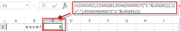
=LOOKUP(2,1/(MID(B1,ROW(INDIRECT("1:"&LEN(B1))),1)="-"),ROW(INDIRECT("1:"&LEN(B1))))

Let’s see how the above formula works:

=ROW(INDIRECT(“1:”&LEN(B1)))

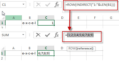
The ROW function will return the row number based on the row references returned by the INDIRECT function. so it will return the below array:

{1;2;3;4;5;6;7;8;9}

=MID(B1,ROW(INDIRECT(“1:”&LEN(B1))),1)

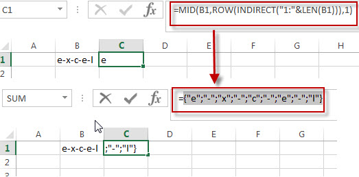
I have talked the above MID function in the previous post to split text string into an array in a cell. So the above formula returns an array like as below:

{"e";"-";"x";"-";"c";"-";"e";"-";"l"}

=MID(B1,ROW(INDIRECT(“1:”&LEN(B1))),1)=”-“

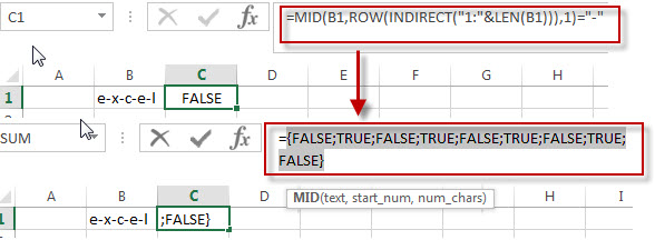
The above formula will check each element in array returned by the above MID function if it is equal to the dash character (“-“). If so, returns TRUE, otherwise, returns FALSE. As it is an array formula, so the above formula should also return an array like as below:

{FALSE;TRUE;FALSE;TRUE;FALSE;TRUE;FALSE;TRUE;FALSE}

=1/(MID(B1,ROW(INDIRECT(“1:”&LEN(B1))),1)=”-“)

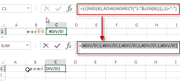
The above formula use 1 to divide each element in the array returned by the MID function. If the value of element in array is TRUE, then returns 1, otherwise, returns a #DIV/0! Error. Just like the below:

{#DIV/0!;1;#DIV/0!;1;#DIV/0!;1;#DIV/0!;1;#DIV/0!}

=LOOKUP(2,1/(MID(B1,ROW(INDIRECT(“1:”&LEN(B1))),1)=”-“),ROW(INDIRECT(“1:”&LEN(B1))))

The LOOKUP function searches for the value of 2 in the first array returned by “1/MID()” formula, you should know that the lookup function can’t find the value of 2 in the first array, so it uses the largest value in the first array that is less than or equal to 2.then returns a value from the same position in the second array returned by the second ROW function.

So the result returned by the above LOOKUP function is the position of the last occurrence of the dash character in Cell B1. It is 8.

You can also use another formula to achieve the same result as follows:

=SEARCH("#",SUBSTITUTE(B1,"-","#",LEN(B1)-LEN(SUBSTITUTE(B1,"-",""))))

Let’s see how the above formula works:

=SUBSTITUTE(B1,”-“,””)

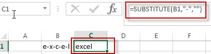
The SUBSTITUTE function will replace all dash characters (“-“) of Cell B1 with empty string.

=LEN(B1)-LEN(SUBSTITUTE(B1,”-“,””))

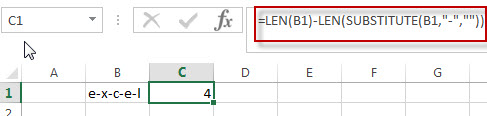
The above formula returns the numbers of dash character in the Cell B1.

=SUBSTITUTE(B1,”-“,”#”,LEN(B1)-LEN(SUBSTITUTE(B1,”-“,””)))

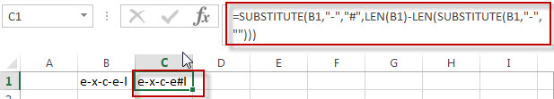
The first SUBSTITUTE function will replace the last occurrence of the dash character with the hash character in Cell B1.

=SEARCH(“#”,SUBSTITUTE(B1,”-“,”#”,LEN(B1)-LEN(SUBSTITUTE(B1,”-“,””))))

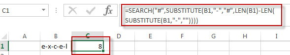
The SEARCH function searches the hash character in a text string returned by the first SUBSTITUTE function, and then returns the position of the hash character. It should be the last occurrence of the dash character in Cell B1.

2. Get the position of Last Occurrence of a character using user defined Function

You can also create a new user defined function to get the position of the last occurrence of a specific character or string in Excel VBA:

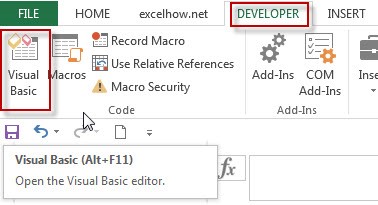
1# click on “Visual Basic” command under DEVELOPER Tab.

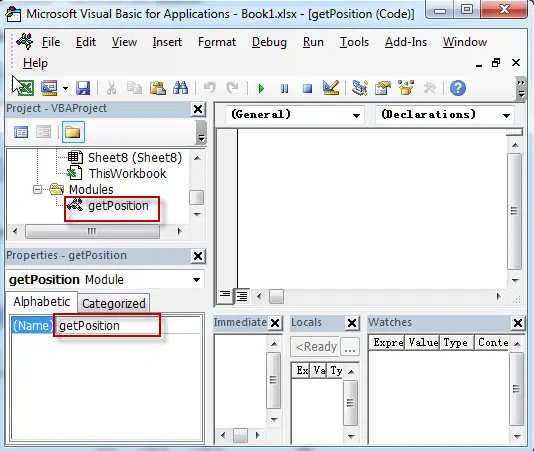
2# then the “Visual Basic Editor” window will appear.

3# click “Insert” ->”Module” to create a new module named as: getPosition

4# paste the below VBA code into the code window. Then clicking “Save” button.

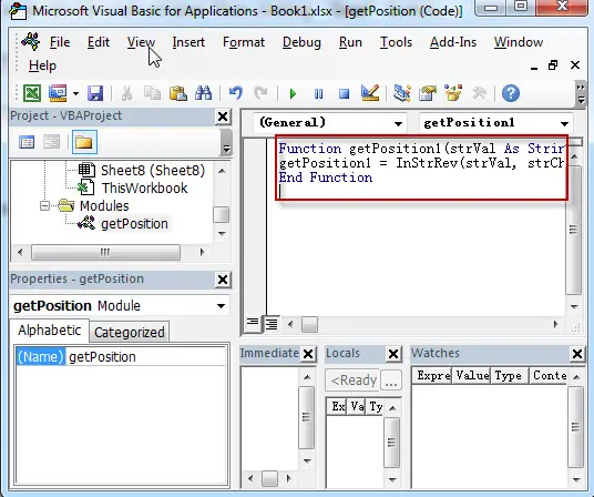
Function getPosition1(strVal As String, strChar As String) As Long
    getPosition1 = InStrRev(strVal, strChar)
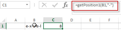
End Function

5# back to the current workbook, then enter the below formula in Cell C1:

= getPosition1(B1,"-")

3. Video: Get the position of Last Occurrence of a character

This Excel video tutorial where we explore two efficient methods to find the position of the last occurrence of a character. In the first method, we’ll dive into a powerful Excel formula, and in the second, we’ll harness the flexibility of VBA scripting.

4. Related Formulas

• Get the position of Last Occurrence of a value in a column
  If you want to find the position number of the last occurrence of a specific value in a column (a single range), you can use an array formula with a combination of the MAX function, IF function, ROW function and INDEX Function.
• Get the Position of the nth Occurrence of a Character in a Cell
  If you want to get the position of the nth occurrence of a character using a excel formula, you can use the FIND function in combination with the SUBSTITUTE function.
• Combine Text from Two or More Cells into One Cell
  If you want to combine text from multiple cells into one cell and you can use the Ampersand (&) symbol.If you are using the excel 2016, then you can use a new function TEXTJOIN function to combine text from multiple cells…
• Split Text String to an Array
  If you want to convert a text string into an array that split each character in text as an element, you can use an excel formula to achieve this result. the below will guide you how to use a combination of the MID function, the ROW function, the INDIRECT function and the LEN function to split a string…
• Find the Relative Position in a Range or Table
  If you want to know the relative row position for all rows in an Excel Range (B3:D6), you can use a excel Array formula as follows:=ROW(B3:D6)- ROW(B3) + 1. You can also use another excel array formula to get the same result as follows:=ROW(B3:D6)-ROW(INDEX(B3:D6,1,1))+1…
• Get the First Row Number in a Range
  If the ROW function use a Range as its argument, it only returns the first row number.You can also use the ROW function within the MIN function to get the first row number in a range. You can also use the INDEX function to get the reference of the first row in a range, then combined to the ROW function to get the first row number of a range.…
•  Get the Last Row Number in a Range
  If you want to get the last row number in a range, you need to know the first row number and the total rows number of a range, then perform the addition operation, then subtract 1, the last result is the last row number for that range.…

5. Related Functions

• Excel ROW function
  The Excel ROW function returns the row number of a cell reference.The ROW function is a build-in function in Microsoft Excel and it is categorized as a Lookup and Reference Function.The syntax of the ROW function is as below:= ROW ([reference])….
• Excel MID function
  The Excel MID function returns a substring from a text string at the position that you specify.The syntax of the MID function is as below:= MID (text, start_num, num_chars)…
• Excel INDIRECT  function
  The Excel ROW function returns the row number of a cell reference.The ROW function is a build-in function in Microsoft Excel and it is categorized as a Lookup and Reference Function.The syntax of the ROW function is as below:= ROW ([reference])….
• Excel LEN function
  The Excel LEN function returns the length of a text string (the number of characters in a text string).The LEN function is a build-in function in Microsoft Excel and it is categorized as a Text Function.The syntax of the LEN function is as below:= LEN(text)…
• Excel LOOKUP function
  The Excel LOOKUP function will search a value in a vector or array.The LOOKUP function is a build-in function in Microsoft Excel and it is categorized as a Lookup and Reference Function.The syntax of the LOOKUP function is as below:= LOOKUP (lookup_value, lookup_vector, [result_vector])…
• Excel Substitute function
  The Excel SUBSTITUTE function replaces a new text string for an old text string in a text string. The syntax of the SUBSTITUTE function is as below:= SUBSTITUTE  (text, old_text, new_text,[instance_num])….
• Excel SEARCH function
  The Excel SEARCH function returns the number of the starting location of a sub-string in a text string. The syntax of the SEARCH function is as below:= SEARCH  (find_text, within_text,[start_num])….