This article will talk about how to create one-dimensional array or two-dimensional array by using some functions in Excel. When using array formulas in Excel, we often use functions to construct arrays.

1. Generate Array with ROW or COLUMN Functions

Array formulas often need to use “natural number” as parameters of the function, such as the second parameter of the LARGE function, OFFSET function in addition to the first parameter. Through the manual way to enter a constant array will be more trouble, and easy to make mistakes. Then we can use the ROW or COLUMN function in EXCEL to generate a sequence, this method is very convenient and fast.

The following formula produces a vertical array of natural numbers from 1 to 10.

{=ROW (1:10)}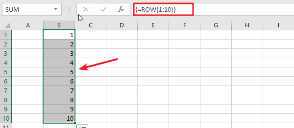

The following formula produces a horizontal array of natural numbers from 1 to 10.

{=COLUMN(A:J)}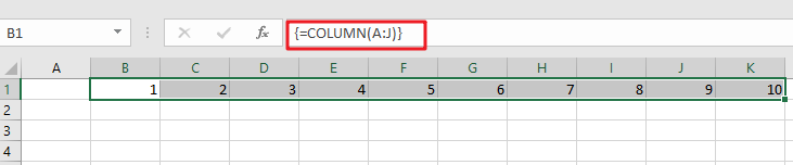

2. Generating two-dimensional Array from one-dimensional Array

Below we will show you how to construct a new two-dimensional array with two columns of data.

a. One-dimensional range rearrangement to generate two-dimensional array

If there is a list of students and the name column of that list contains 10 students’ names, we need to randomly place the students’ names in the name column into the cell range of 5 rows and 2 columns (a new two-dimensional array).

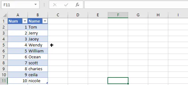
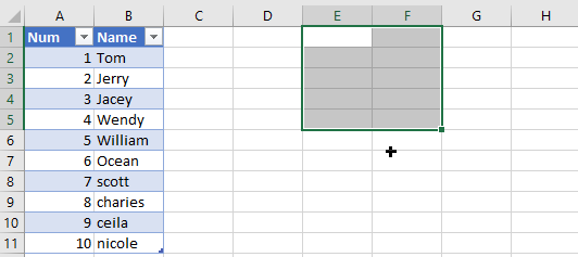
We can use the following steps to randomize the names of students in column B to a 5 row 2 column range, such as the cell range E1:F5.

STEP1# Select the cell range E1:F5

STEP2# Enter the following array formula in the formula bar

=INDEX(B2:B11,RIGHT(SMALL(RANDBETWEEN(A2:A11^0,999)/1%+A2:A11,ROW(1:5)*2-{1,0}),2))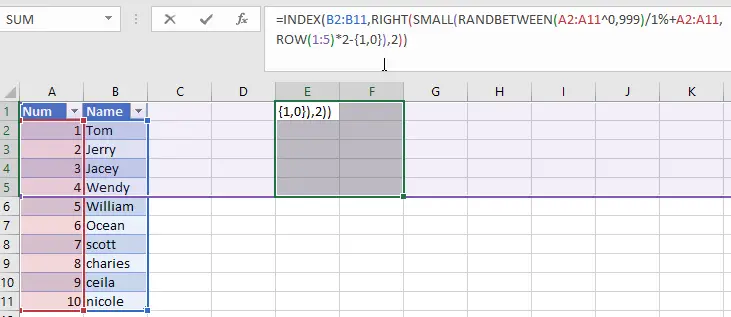

STEP3# Press CTRL + SHIFT +ENTER shortcut keys to convert the above formula into an array formula.

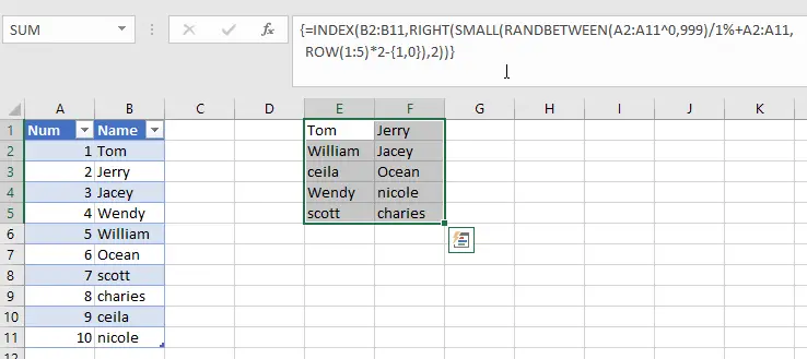
STEP4# You will see that the students’ names have been randomly placed in a two-dimensional range of array.

Let’s see how this array formula works.

=RANDBETWEEN(A2:A11^0,999)

The RANDBETWEEN function is used to generate an array of 10 values, where the elements are random integers between 1 and 1000. Since the elements are randomly generated, the size of the array elements is randomly ordered. The array formula generates an array of random integers as follows.

={484;203;468;525;702;220;13;163;386;54}

=RANDBETWEEN(A2:A11^0,999)/1%+A2:A11

The random integer array generated above is multiplied by 100 and then added to the ordinal array of 1 to 10. This ensures that the last two digits of the array elements are ordinal numbers 1 to 10.

={484;203;468;525;702;220;13;163;386;54}/1%+A2:A11

The above array formula returns the following array:

{48401;20302;46803;52504;70205;22006;1307;16308;38609;5410}

=ROW(1:5)*2-{1,0}

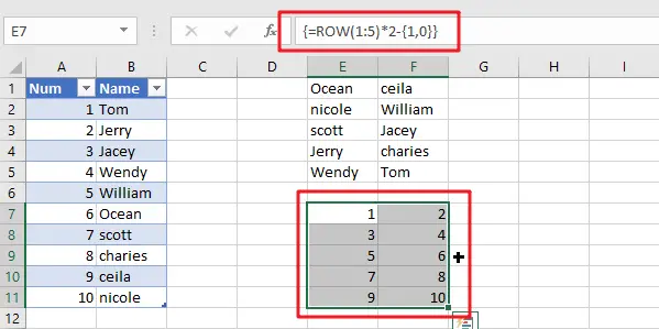
The ROW function generates a vertical array {1;2;3;4;5), and then subtracts a constant array {1,0} to produce a two-dimensional array of 5 rows and 2 columns.

=SMALL()

The result is taken as the second argument to the SMALL function, which sorts the array after multiplication and addition processing. Since the original size of the array is random, after sorting, the ordinal number corresponding to the last two digits of each element is randomly ordered.

=RIGHT()

The RIGHT function is used to extract the last two digits of each element, and the INDEX function is used to return the student’s name in the corresponding position in column B. In this way, the names in column B can be randomly populated into a two-dimensional array of 5 rows and 2 columns.

b. Combining two columns of data to create a two-dimensional array

We can use the VLOOKUP function to query from the right to the left, and we can use the array operation and IF function to swap two columns of data to generate a new two-dimensional array.

Here is an example of how the VLOOKUP function can be used to reverse the query by constructing a new array.

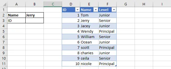
If you have a table of employee information, and you need to find the employee’s number by the employee’s name, you can use the VLOOKUP function in combination with the IF function to construct a two-dimensional array to find the corresponding employee number.

The employee information table is as follows:

To find the employee number by name, the steps are as follows.

STEP1# Select the cell B3

STEP2# Enter the following formula in the formula bar and press Enter

=VLOOKUP(B2,IF({1,0},E2:E11,D2:D11),2,)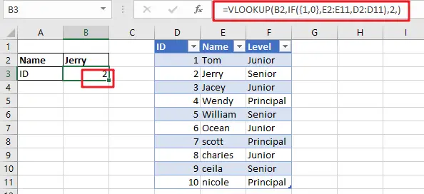

STEP3# As you can see, Jerry’s employee number has been found.

Let’s see how the above formula works.

The core part of the formula is IF ({1,0},E2:E11,D2:D11), which uses a horizontal array {1,0} and two vertical arrays to perform operations to achieve the position of the column where the employee’s name and work number are swapped. Its returned memory arrays are：

{"Tom",1;"Jerry",2;"Jacey",3;"Wendy",4;"William",5;"Ocean",6;"scott",7;"charies",8;"ceila",9;"nicole",10}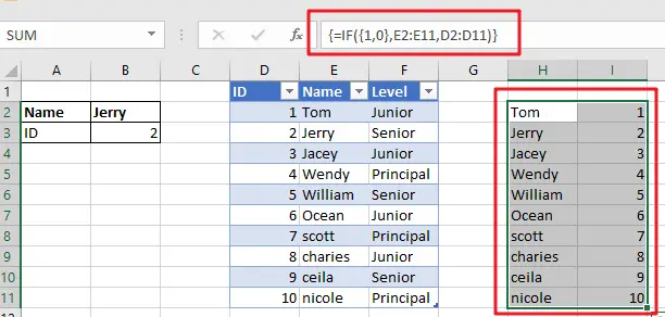

The VLOOKUP function then queries the employee’s name in the two-dimensional array generated by the IF function and returns the corresponding employee number.

3. Extracting Sub-arrays From Data

In daily work, it is often necessary to extract part of the data from a column and reprocess it. For example, If you want to find out the list of employees who meet the specified requirements in the employee table.

The following describes how to extract some data from a column to form a subarray.

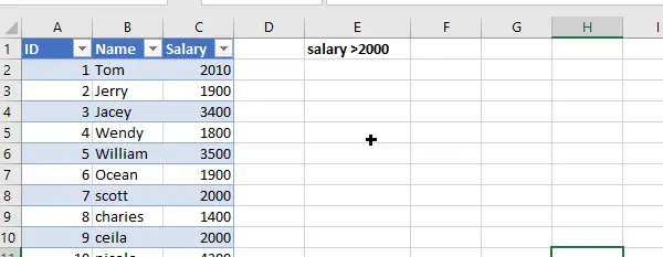
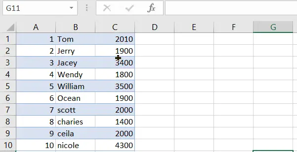
Suppose you have an employee salary table and you want to find out the names of employees whose salary is greater than $2000. The salary table is as follows.

You can refer to the following steps to obtain a list of employees who meet the requirements.

STEP1# First you need to select the cell range E2:E11

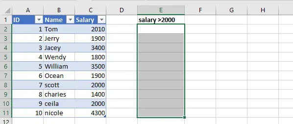
STEP2# Enter the following formula in the formula bar

=T(OFFSET(B1,SMALL(IF(C2:C11>2000,A2:A11),ROW(INDIRECT("1:"&COUNTIF(C2:C11,">2000")))),))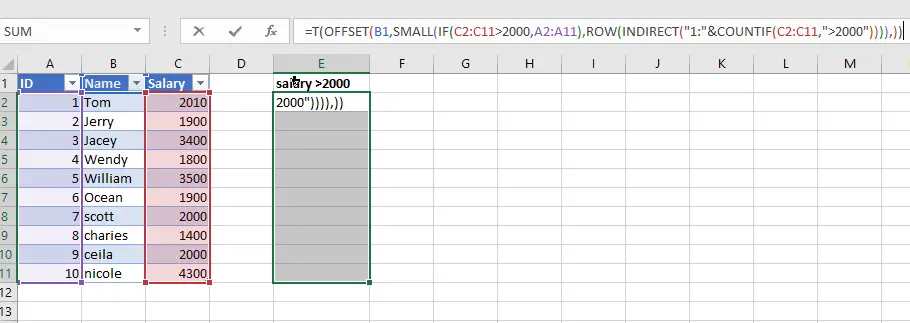

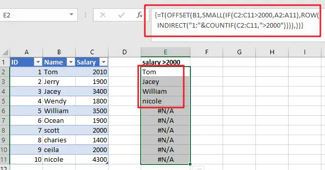
STEP3# Press CTRL + SHIFT +ENTER shortcut keys to convert the above formula into an array formula.

Let’s see how the above formula works.

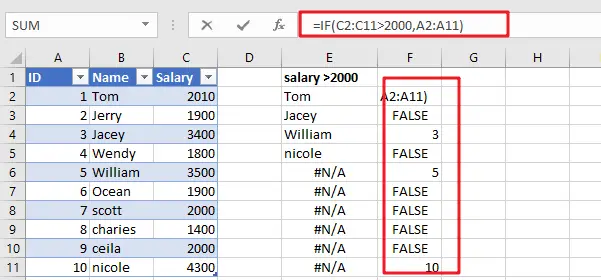
=IF(C2:C11>2000,A2:A11)

First use the IF function to determine whether the salary meets the conditions, if the salary is greater than $2000, then return the employee’s ID, otherwise return the logical value FALSE.

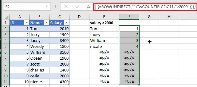
=ROW(INDIRECT(“1:”&COUNTIF(C2:C11,”>2000″)))

The COUNTIF function is used to calculate the number of scores greater than 100 and is combined with the ROW function and INDIRECT function to generate a sequence of natural numbers from 1 to n.

=SMALL(IF(C2:C11>2000,A2:A11),ROW( INDIRECT(“1:”&COUNTIF(C2:C11,”>2000″))))

Use the SMALL function to find the employee number whose salary is greater than $2000 and return the following memory array.

={1;3;5;10}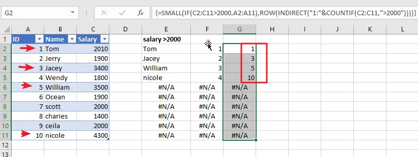

=OFFSET(B1,{1;3;5;10},)

The OFFSET function extracts the employee’s name from the result returned by the SMALL function and returns the following array of employee names.

={"Tom";"Jacey";"William";"nicole"}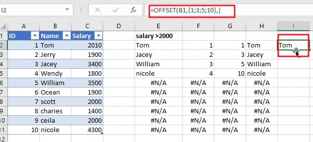

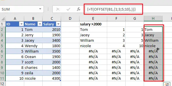
=T(OFFSET(B1,{1;3;5;10},))

Finally, the T function is used to convert the multi-dimensional reference returned by the OFFSET function into a memory array.

4. Extracting Sub-array from a two-dimensional Array

The cell range A1:C10 contains data of text and numeric type, see the figure below.

If you want to extract all the text-based data from the specified cell range A1:C10, then you can use the following array formula.

=T(INDIRECT(TEXT(SMALL(IF(A1:C10>="",ROW(A1:C10)/1%+COLUMN( A1:C10)),ROW(INDIRECT("1:"&COUNTIF(A1:C10,"*")))), "r0c00"),))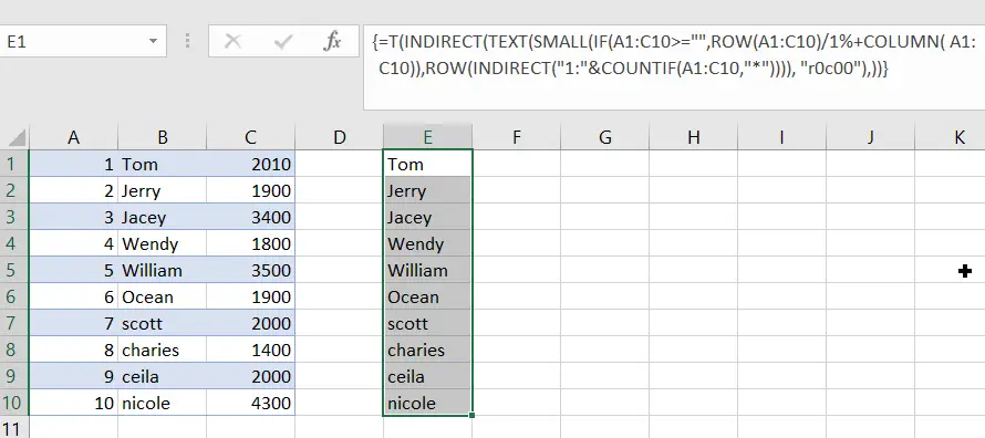

Let’s see how the above formula works.

=IF(A1:C10>=””,ROW(A1:C10)/1%+COLUMN( A1:C10))

The IF function is used to determine the type of data in the cell range. If the cell value is the text, then let the cell’s line number multiplied by 100, and then add the cell’s column number, and then return a numeric result; if the cell value is not text type, then return the logical value FALSE.

={FALSE,102,FALSE;FALSE,202,FALSE;FALSE,302,FALSE;FALSE,402,FALSE;FALSE,502,FALSE;FALSE,602,FALSE;FALSE,702,FALSE;FALSE,802,FALSE;FALSE,902,FALSE;FALSE,1002,FALSE}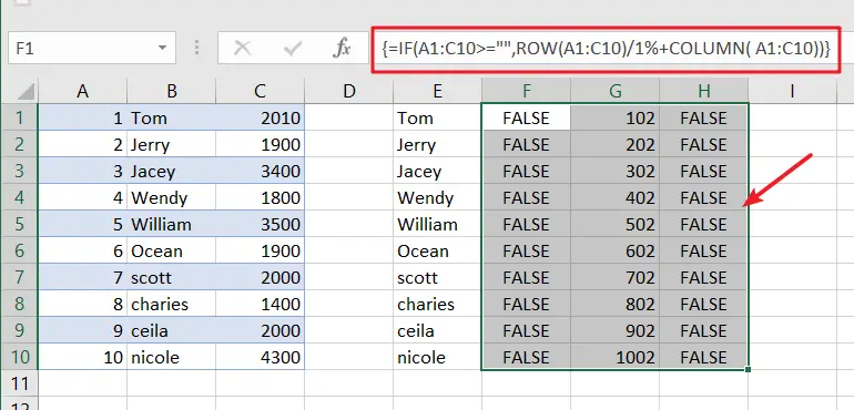

=ROW(INDIRECT(“1:”&COUNTIF(A1:C10,”*”)))

The COUNTIF function is used to calculate the number of text values in the range of cells A1:C10, and combined with the ROW function and INDIRECT function to generate a series of natural numbers from 1 to n.

={1;2;3;4;5;6;7;8;9;10}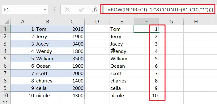

=SMALL(IF(A1:C10>=””,ROW(A1:C10)/1%+COLUMN( A1:C10)),ROW(INDIRECT(“1:”&COUNTIF(A1:C10,”*”))))

The SMALL function is used to extract the position information of the cell where the text is located and return a memory array.

={102;202;302;402;502;602;702;802;902;1002}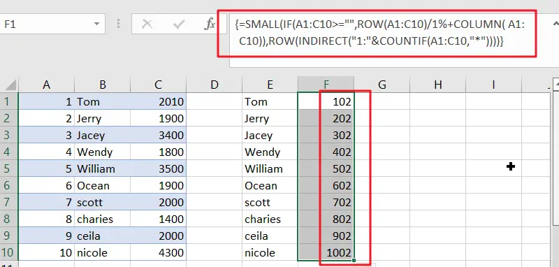

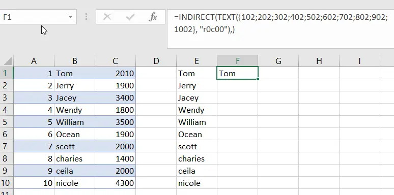
=INDIRECT(TEXT({102;202;302;402;502;602;702;802;902;1002}, “r0c00”),)

The TEXT function is used to convert the location information to R1C1 reference style, and then use the INDIRECT function to return to the cell reference.

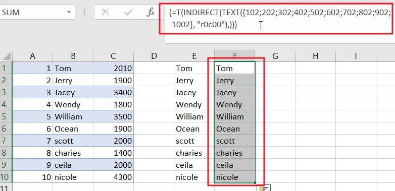
=T(INDIRECT(TEXT({102;202;302;402;502;602;702;802;902;1002}, “r0c00”),))

Finally, the multi-dimensional references returned by the INDIRECT function are converted to memory arrays using the T function.

5. Fill the Merged Cells by Array Formula

In the merged cells, only the first cell has a value, while the rest of the cells are empty cells. When we work with the data, we may need to fill the empty cells in the merged cells with the corresponding values to meet the needs of the calculation.

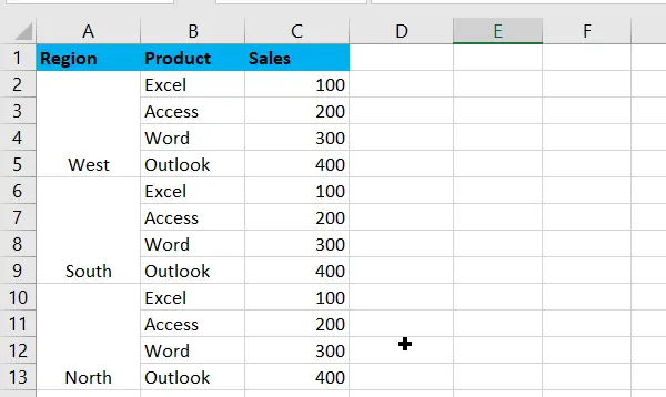
The following is a product sales table, we need to fill the empty cells in the merged cells with the corresponding region name. The data table is as follows:

You can fill the data into the merged cells by using the following array formula.

=LOOKUP(ROW(A2:A13),ROW(A2:A13)/(A2:A13>""),A2:A13)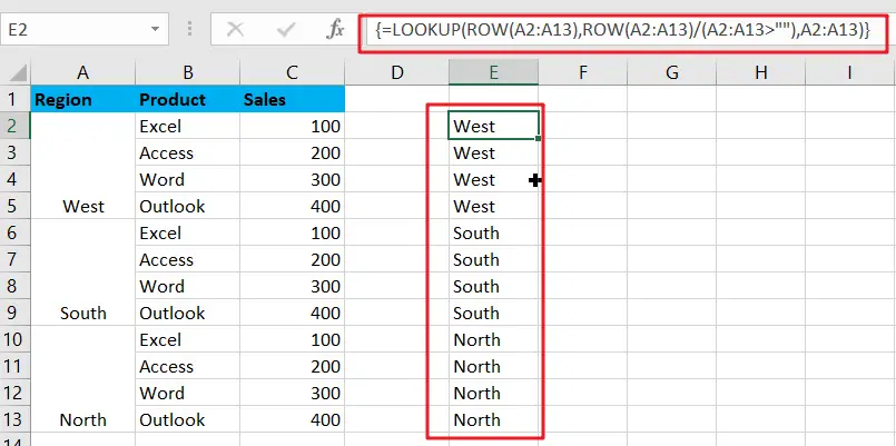

Let’s See How This Formula Works:

=ROW(A2:A13)/(A2:A13>””)

This formula assigns a non-empty cell in column A to the row number of that cell, and returns the error value #DIV/O! for empty cells, and finally returns a memory array.

{2;#DIV/0!;#DIV/0!;#DIV/0!;6;#DIV/0!;#DIV/0!;#DIV/0!;10;#DIV/0!;#DIV/0!;#DIV/0!}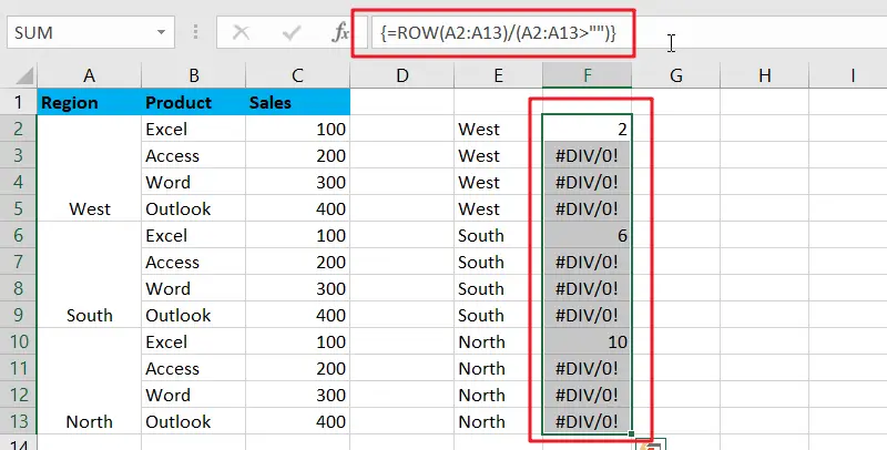

Finally, the LOOKUP function is used to perform a fuzzy search and return the corresponding region name.

6. Convert Two-dimensional Array to one-dimensional Array

Some functions only support one-dimensional array as their arguments, not two-dimensional array. For example, the second argument of the MATCH function, the second argument of the LOOKUP function, and so on. If you want to complete the query in a two-dimensional array, you need to first convert the two-dimensional array to a one-dimensional array.

In the figure below, the cell range A1:C4 is a two-dimensional array, by using the following formula you can return the maximum value less than or equal to 100 in the cell range; LOOKUP function will perform a fuzzy search from a one-dimensional array returned by the SMALL formula, and return the value that matches the conditions.

The formula is as follows.

=LOOKUP(100,SMALL(A1:C4,ROW(1:12)))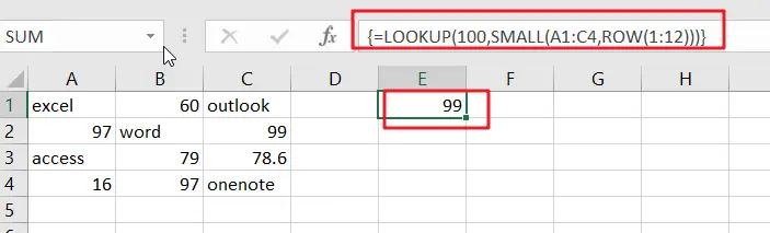

Let’s see how this formula works:

=SMALL(A1:C4,ROW(1:12))

Because the cell range is 4 rows and 3 columns, it is a two-dimensional array containing 12 elements. You can generate a sequence of natural numbers from 1 to 12 by using the ROW function. Then use the SMALL function to sort the two-dimensional array and return a one-dimensional memory array. The result is as follows:

={16;60;78.6;79;97;97;99;#NUM!;#NUM!;#NUM!;#NUM!;#NUM!}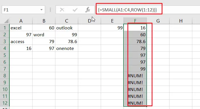

The LOOKUP function performs a fuzzy lookup by row and ignores the error value #NUM!. Finally, the maximum value less than or equal to 100 is returned, which is 99.