In Microsoft Excel Spreadsheet or Google sheets, there is another cell reference, mixed references, where part of the reference is absolute, part of the relative. This article will describe how to use mixed references through specific examples.
Table of Contents
Mixed Reference
When the formula is copied to other cells, it is only used to maintain the absolute position of one of the rows or columns of the referenced cell in Excel or Google Sheets, while the direction of the other positions are changed, this type of reference is called mixed references.
Mixed references can be categorized into absolute column and relative row(=$A1) and relative column and absolute row(=A$1) references.
For example: formula: =$B1, when the formula is copied to the right, it will always keep $B1 unchanged, and the row number will change when copied down, that is, row relative and column absolute references.
EXAMPLE
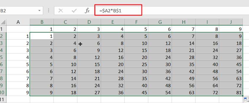
If you have a table in which the B1:J1 cell range entered the number 1-9, A2:A10 cell range also entered 1-9, we want to calculate the intersection of B1: J1 and A2: A10 two cell range of cell multipliers, this time, you have to use a mixed reference. You can enter the following mixed reference formula in cell B2.
=$A2*B$1
If you want to be able to fix a cell address when copying a formula, then simply use the absolute reference symbol $ before the row or column number.
Quickly toggle between reference types
The shortcut keys F4 or Fn+F4 are provided in both Excel and Google Sheets to toggle between different reference types. For the formula = A1, press F4 or Fn+F4 to switch the order of the shortcut keys as follows.
$A$1->A$1->$A1->A1
Video: Excel/Google Sheets: Mixed Reference
SAMPLE FILE
Below are sample files in Microsoft Excel and Google sheets that you can download for reference if you wish.
Google Sheets Sample file: click here.