This post will guide you how to make chart X Axis labels to display below negative in Excel. How do I move X Axis labels to bottom on your chart in Excel. How to make the chart X Axis go on the bottom of the chart in Excel.
Table of Contents
1. Move X Axis to Bottom for Negative Data
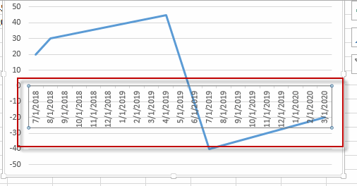
When you created a bar chart or line chart in your worksheet, and the X Axis labels are stuck at 0 position of the Axis. And if you source data have negative values, and you want to move X Axis labels below negative, how to achieve it. Let’s see the below detailed steps.
Step1: click the X Axis to select it.

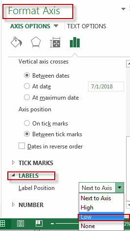
Step2: right click on the selected X Axis, and select Format Axis… from the pop-up menu list. The Format Axis pane will be displayed in the right of excel window.
Step3: on Format Axis pane, expand the Labels section, select Low option from the Label Position drop-down list box. Close the Format Axis pane.

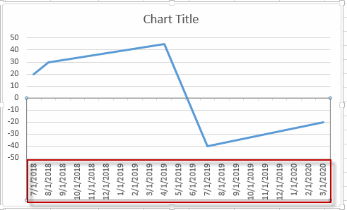
Step4: you will see that the X-Axis labels have been moved to bottom of the chart.

2. Video: Make Chart X Axis Labels Display below Negative Data
If you want to learn how to make chart X Axis labels display below negative values in Excel, you can watch this video for a step-by-step guide.
Leave a Reply
You must be logged in to post a comment.