This post will teach you how to highlight rows in a table with conditional formatting in Excel. You will learn that how to change the color of the entire rows if the value of cells in a specified column meets your conditions, such as, if the value of cells is equal to or greater than a certain number or text values, then excel should be highlight entire rows or change a row color as you need.
Highlight rows based on a numeric value
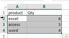
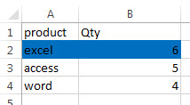
Assuming that you have a table in range, and you want to highlight rows in that table where the value of cells in column B is greater than 5, and then you need to create the Conditional Formatting Rules and use a formula to apply conditional formatting, here you can use the formula:
=$B1>5
Let’s see the below detailed steps:
1# select the range of cells in your table
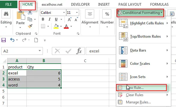
2# on the HOME tab, click the Conditional Formatting command under Styles group. Then select New Rules… from the drop-down menu list.
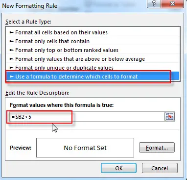
3# the New Formatting Rule window will appear.
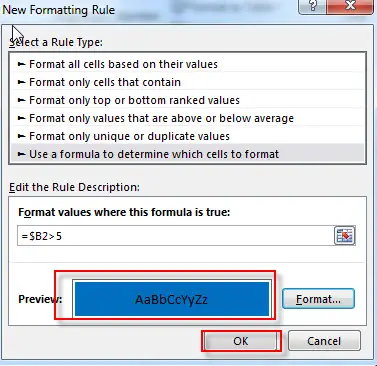
4# select the Use a formula to determine which cells to format option under Select a Rule Type: box, and then enter the following formula in the Format values where this formula is true: box: =$B2>5
Note: you can create your formulas to check a cell if meet your conditions. Such as, you can change the condition as $C2<0.
You also need to notice that the dollar sign $ before the cell’s reference, you need to keep it when the formula need to check in a specified column.
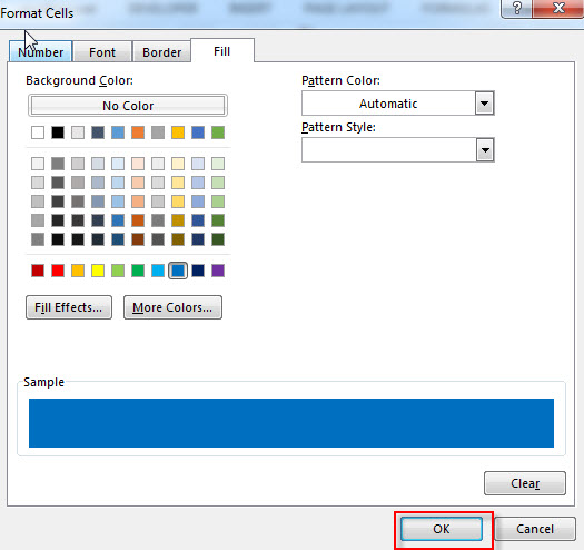
5# click the Format… button, then the Format Cells window will appear.
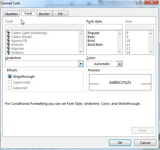
6# in the “Format Cells” window, switch to the Fill tab, choose the background color, and then click OK button. You can also switch to other tabs to tweak the settings as you want.
7# back in the New Formatting Rule window, you can see a preview of your rows background color. Then click OK button.
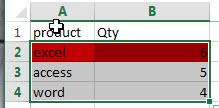
8# you can see that the conditional formatting are beginning to take effect.
Note:
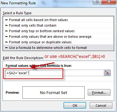
If you want to highlight rows based on a text value, you can use the following generic formula to apply conditional formatting:
=$A2=”excel”
or
=SEARCH(“excel”,$B1)>0
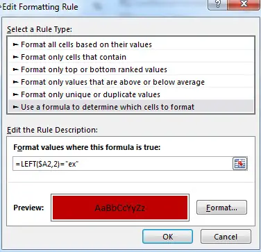
If you want to change a row color if the cell value in a specified column begin with a specific character or text string, you can use the following formula as the conditional formatting rule.
=LEFT($A2,2)=”ex”
So you can create additional formulas for your complex needs.
Related Functions
- Excel SEARCH function
The Excel SEARCH function returns the number of the starting location of a substring in a text string.The syntax of the SEARCH function is as below:= SEARCH (find_text, within_text,[start_num])… - Excel LEFT function
The Excel LEFT function returns a substring (a specified number of the characters) from a text string, starting from the leftmost character.The LEFT function is a build-in function in Microsoft Excel and it is categorized as a Text Function.The syntax of the LEFT function is as below:= LEFT(text,[num_chars])…t)…
Related Posts
- Highlight Duplicate Rows
this post will talk that how to highlight entire rows that are duplicates in excel 2016, 2013 or lower version. Or how to change the background color of duplicate rows..… - Find Duplicate Rows
If you want to check the entire row that duplicated or not, if True, then returns “duplicates” value, otherwise, returns “no duplicates”. You can create a formula based on the IF function and the SUMPRODUCT function… - Highlight duplicate values
this post will teach you how to highlight duplicate values in the range of cells in excel. Normally, you may be need to identify duplicate values with a range of cells in Excel. And there is one of the fasted way that is using conditional formatting feature in Microsoft Excel…… - Combine Duplicate Rows and Sum the Values
This post will teach you how to combine duplicate rows and sum the corresponding values or calculate numbers in specific column in excel. And how to merge duplicate rows and then sum the values with VBA macro in Excel..…
Leave a Reply
You must be logged in to post a comment.