This post will guide you how to find and replace multiple values at once with VBA macro or using formula  in Excel. How do I make multiple find and replace in Excel.

Suppose that you have a few cells containing few values and you want to find and replace two or three values; then you might think that it’s not a big deal; because you would prefer to do it with the help of the Find and Replace built-in feature of excel, then congratulation because you have supposed to choose the right way for this task.

There isn’t any doubt that you can find and replace values in excel by its Find and Replace built-in feature, which works entirely perfect for two or three values, but when you would have the bulk of values, and you want to find and replace them, then doing this task manually by the aid of this Find and Replace built-in feature would be a stupid decision because you would get tired of it and would never complete your work on time.

But there isn’t any need to worry about it because, luckily, there are a few effective methods for finding and replacing multiple values in a few seconds.

After reading this article carefully, you would get to know the several ways to find and replace multiple words, individual characters, or strings so that you can select the best one according to your needs and ease.

So let’s get straight into it!

1. Find and Replay Multiple Values using Formula

 General formula:

The formula given below would help you out for finding and replacing multiple values within few seconds:

=SUBSTITUTE(SUBSTITUTE(B2,INDEX(finding_values,1),INDEX(replacing_values,1)),INDEX(finding_values,2),INDEX(replacing_values,2))

or

=SUBSTITUTE(SUBSTITUTE(B2,finding_values,replacing_values), finding_values, replacing_values))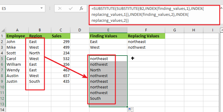

Syntax Explanation:

Before we dive into the formula for getting the job done effectively, we need to understand each syntax so that we can know how each syntax helps to find and replace the multiple values:

• SUBSTITUTE: This function lets users replace current text in a text string with new text when they desire to replace text based on its content rather than its position.
• INDEX: The INDEX function in Excel is used to repeat characters a specified number of times.
• B2: This is the input value.
• Find: This command specifies the text to be found in the input range.
• Replace: It represents the text that is being replaced.
• The comma sign (,): is a separator that may separate a list of values.
• Parenthesis (): The primary purpose of the parenthesis () symbol is to organize the components.

Let’s See How This Formula Works:

As I said above, there are a few ways to find and replace multiple values in Excel in a matter of seconds, and one of the most popular and simple methods is to utilize the nested SUBSTITUTE function.

The logic of this formula is very simple: you write a few individual functions to replace an old value with a new one. Then you nest those functions one inside the other so that each subsequent SUBSTITUTE uses the output of the previous SUBSTITUTE to find the next value.

=SUBSTITUTE(SUBSTITUTE(Text_values,finding_values,replacing_values), finding_values, replacing_values))

Assume you wish to replace the region names in the B2:B9 list of places with the replacing names.

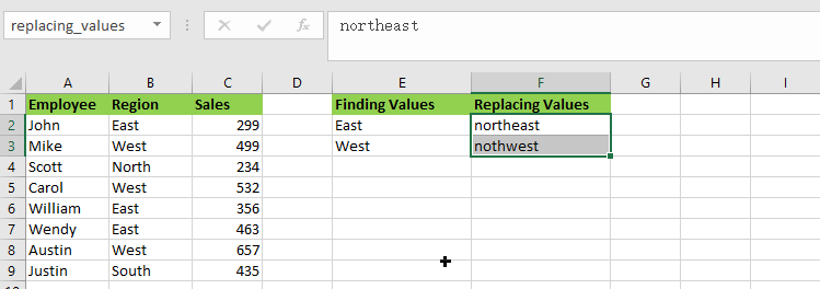
For getting the desired output, input the old values in E2:E3 and the new values in F2:F3, as seen in the image and formula below. Then, in E5, enter the following formula:

= SUBSTITUTE(SUBSTITUTE(B2, E2, F2), E3,F3)

You’ll have completed all of the replacements at once:

Please remember that the above method only works in Excel 365, which supports dynamic arrays.

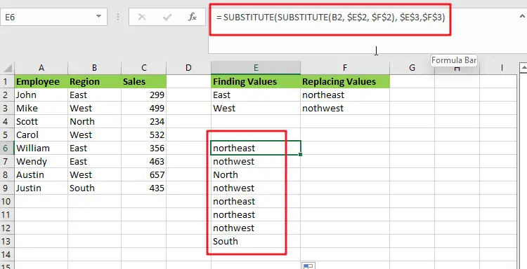
In pre-dynamic versions of Excel 2016, Excel 2019, and prior,type the following formula:

= SUBSTITUTE(SUBSTITUTE(B2, $E$2, $F$2), $E$3,$F$3)

Also, note that in this case, we lock the replacement values with absolute cell references to ensure that they do not shift when copying the formula down.

The SUBSTITUTE function is case-sensitive, so you must type the old values (old text) in the same letter case as the original data.

This method has a significant drawback: It should only be used for a limited number of find/replace values. This nested function becomes extremely difficult to manage when you have dozens of values to replace.

Benefits: Simple to deploy; compatible with all Excel versions

2. Find and replace multiple values using XLOOKUP Function

The XLOOKUP function is very efficient and helpful while replacing the entire cell content rather than just a portion of it.

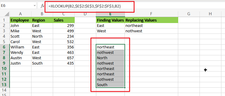
Assume you have a list of region in column B and want to replace all the “East” or “West” regions as “northeast” or “northwest” values. Enter the following formula in B2:

=XLOOKUP(B2,$E$2:$E$3,$F$2:$F$3,B2)

The formula does the following when translated from Excel to human language:

It searches the B2 value (lookup value) in E2:E3 (lookup array) and returns a match from F2:F3 (return array). If the original value cannot be retrieved, take it from B2.

Because the XLOOKUP function is only accessible in Excel 365. However, you can easily replicate this behavior using a combination of IFERROR or IFNA and VLOOKUP:

=IFNA(VLOOKUP(B2,$E$2:$F$3,2,FALSE),B2)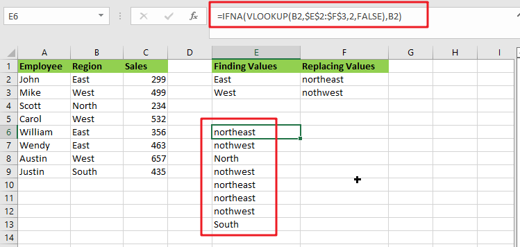

Unlike the SUBSTITUTE, the XLOOKUP and VLOOKUP functions are both not case-sensitive, which means they search for lookup values regardless of letter case.

 3. Find And Replace Multiple Values with VBA Macro

Assuming that you have a list of data in range B1:B6, and you want to find multiple values and replace those value with different values. For example, find “excel” string and replace its as excel2013, and find “word’’ string and replace its as word2013, and so on. How to achieve it. You should use an excel VBA macro to quickly find and replace multiple values. Just do the following steps:

#1 open your excel workbook and then click on “Visual Basic” command under DEVELOPER Tab, or just press “ALT+F11” shortcut.

#2 then the “Visual Basic Editor” window will appear.

#3 click “Insert” ->”Module” to create a new module.

#4 paste the below VBA code into the code window. Then clicking “Save” button.

Sub ReplaceMulValues()
    Dim myRange As Range, myList As Range
    Set myRange = Application.Selection
    Set myRange = Application.InputBox("Select one range to be searched", "Find And Replace Multiple Values", myRange.Address, Type:=8)
    Set myList = Application.InputBox("select two column range where find/replace pairs are:", "Find And Replace Multiple Values", Type:=8)
    For Each cel In myList.Columns(1).Cells
        myRange.Replace what:=cel.Value, replacement:=cel.Offset(0, 1).Value
    Next
End Sub

#5 back to the current worksheet, then run the above excel macro. Click Run button.

#6 Select one range to be searched

#7 select two column range where find/replace pairs are

#8 let’s see the result.

4. Video: Find and Replace Multiple Values

This Excel video tutorial, where we’ll explore two methods -—leveraging the VLOOKUP function and utilizing VBA Macro—for efficiently find and replace multiple values.

5. Related Functions

• Excel Substitute function
  The Excel SUBSTITUTE function replaces a new text string for an old text string in a text string. The syntax of the SUBSTITUTE function is as below:= SUBSTITUTE  (text, old_text, new_text,[instance_num])….
• Excel IFERROR function
  The Excel IFERROR function returns an alternate value you specify if a formula results in an error, or returns the result of the formula.The syntax of the IFERROR function is as below:= IFERROR (value, value_if_error)….
• Excel VLOOKUP function
  The Excel VLOOKUP function lookup a value in the first column of the table and return the value in the same row based on index_num position.The syntax of the VLOOKUP function is as below:= VLOOKUP (lookup_value, table_array, column_index_num,[range_lookup])….
• Excel INDEX function
  The Excel INDEX function returns a value from a table based on the index (row number and column number)The INDEX function is a build-in function in Microsoft Excel and it is categorized as a Lookup and Reference Function.The syntax of the INDEX function is as below:= INDEX (array, row_num,[column_num])…
• Excel XLOOKUP function
  This tutorial will show you how to filter out or extract the top n values from the list having few values using Filter function or XLookup function in Excel The syntax of the xlookup function is as below:=XLOOKUP(lookup value, lookup array, return array, [if not found], [match mode], [search mode])…