As an MS Excel user, you might have come across a task in which you need to calculate the average values of the last 2 numeric values, and you might have done this task manually but suppose if the last values you want to calculate the average exceeds to 3, 5 or N numeric values then what would you do? If you would tend to do this task manually, then it would be your foolish decision because doing these kinds of lengthy tasks manually is very hard, and when it comes to N numeric values, then It would not be wrong to say that this is near to impossible to do it manually.

But don’t worry about it because after carefully reading this article, you can easily calculate the average values of the last 3, 5, and most important N numeric values within seconds.

So without any further delay, let’s dive into it;

Calculate The Average Of The Last 3 Values In MS Excel

The General Formula is as below based on the AVERAGE function, LOOKUP function, LARGE function and IF function:

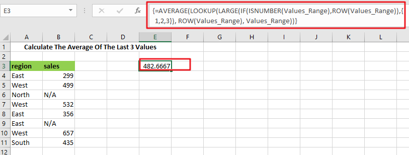
=AVERAGE(LOOKUP(LARGE(IF(ISNUMBER(Values_Range),ROW(Values_Range)),{1,2,3}),ROW(Values_Range), Values_Range))

Note: this above is an array formula, you need to press “CTRL+SHIFT+ENTER” short cuts to make it as array formula.

 Let’s See How This Formula Works

You can use an array formula for getting the average of the last 3 values in the range. The formula in E3 in the example is as follows:

=AVERAGE(LOOKUP(LARGE(IF(ISNUMBER(Values_Range),ROW(Values_Range)),{1,2,3}), ROW(Values_Range), Values_Range))

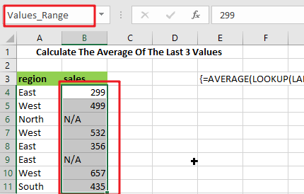
Here “ Values_Range ” refers to the designated name range B4:B11.

This is an array formula, so input it using control + Shift + enter.

Because the AVERAGE function computes an average of numbers supplied in an array, practically all of the effort in this formula is to construct an array of the latest three numeric values in a range.

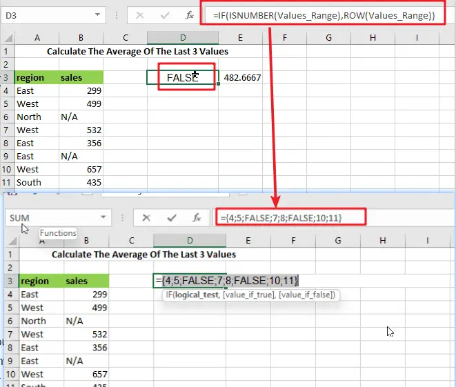
 =IF(ISNUMBER(Values_Range),ROW(Values_Range))

The IF function in the formula is used to “filter” numeric numbers from the inside out.

Because the ISNUMBER function returns TRUE for numeric values and FALSE for other values (including blanks), and the ROW function produces row numbers, the outcome of this operation is an array of row numbers corresponding to numeric entries:

={4;5;FALSE;7;8;FALSE;10;11}

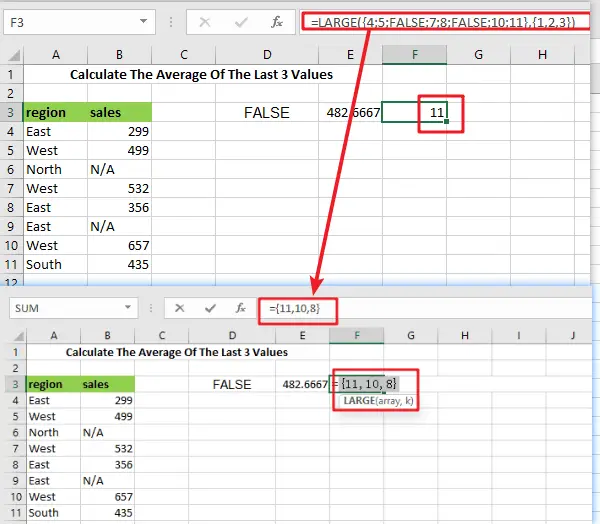
=LARGE({4;5;FALSE;7;8;FALSE;10;11},{1,2,3})

The above array is sent to the LARGE function, using the array constants 1,2,3 for k. LARGE ignores FALSE values and returns an array with the greatest three integers, which correspond to the last three rows with numeric values:

={11,10,8}

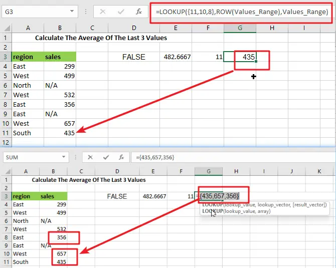
=LOOKUP({11,10,8}, ROW(Values_Range), Values_Range))

The above array is used as the lookup value in the LOOKUP function. The ROW function provides the lookup array, and the return array is the named range “ Values_Range “:

={435,657,356}

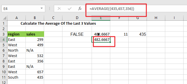
The array of similar values in “ Values_Range ” returned by LOOKUP is then put into AVERAGE:

=AVERAGE({435,657,356})

Calculate The Average Of The Last 5 Values IN MS Excel

Please use the following array formula, which would assist you in calculating the last 5 values in MS Excel:

In a blank cell, type the following formula:

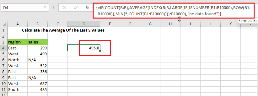
=IF(COUNT(B:B),AVERAGE(INDEX(B:B,LARGE(IF(ISNUMBER(B1: B10000),ROW(B1: B10000)),MIN(5,COUNT(B1: B10000)))):B10000),"no data found") 

Note: B:B is the column that holds the data you used, B1: B10000 is a dynamic range that you may stretch as long as you need, and the number 5 represents the latest n values, and then press Ctrl + Shift + Enter to make the formula as array formula to obtain the average of the last 5 numbers. See the following screenshot:

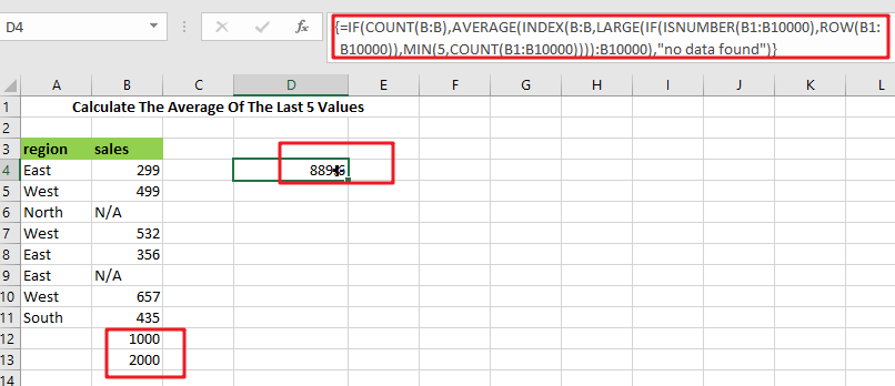
And now, when you enter new numbers underneath the old data, the average is updated as well, as seen in the screenshot:

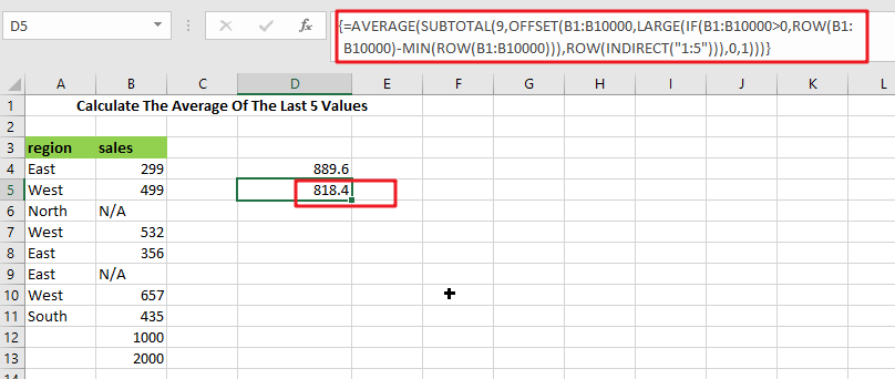
Note: If the column of cells contains 0 values and you want to exclude the 0 values from your last 5 numbers, the above formula will not work. Instead, I can introduce you to another array formula that will retrieve the average of the last 5 non-zero values; please input this formula:

=AVERAGE(SUBTOTAL(9,OFFSET(B1:B10000,LARGE(IF(B1:B10000>0,ROW(B1:B10000)-MIN(ROW(B1:B10000))),ROW(INDIRECT("1:5")),0,1)))

Then press Ctrl + Shift + Enter to achieve the desired result, see screenshot:

Calculate The Average Of The Last N Values In MS Excel

In Excel, you can use the AVERAGE function in conjunction with the OFFSET and COUNT functions to determine the average for the last N values. This article will demonstrate how to use Excel’s basic formulae to determine the average of the last N data.

General Formula:

In Excel, use the formula below to calculate the average of the last N values.

=AVERAGE(OFFSET(B1,COUNT(B:B),0,-N))

Explaination

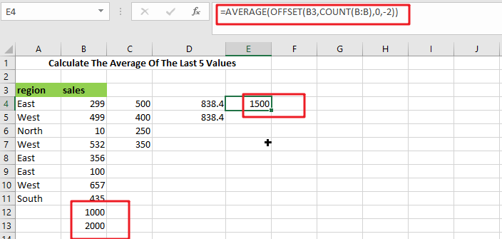
In the example figure below, we’ll place the input values in Column C and want to get the average of the last two values.

Then, in the formula bar section, enter the formula as below:

=AVERAGE(OFFSET(B3,COUNT(B:B),0,-2))

Finally, the result will be shown in cell E2.

Related Functions

• Excel ROW function
  The Excel ROW function returns the row number of a cell reference.The ROW function is a build-in function in Microsoft Excel and it is categorized as a Lookup and Reference Function.The syntax of the ROW function is as below:= ROW ([reference])….
• Excel IF function
  The Excel IF function perform a logical test to return one value if the condition is TRUE and return another value if the condition is FALSE. The IF function is a build-in function in Microsoft Excel and it is categorized as a Logical Function.The syntax of the IF function is as below:= IF (condition, [true_value],
• Excel ISNUMBER function
  The Excel ISNUMBER function returns TRUE if the value in a cell is a numeric value, otherwise it will return FALSE.The syntax of the ISNUMBER function is as below:= ISNUMBER (value)…
• Excel LOOKUP function
  The Excel LOOKUP function will search a value in a vector or array.The syntax of the LOOKUP function is as below:= LOOKUP (lookup_value, lookup_vector, [result_vector])…
• Excel AVERAGE function
  The Excel AVERAGE function returns the average of the numbers that you provided.The syntax of the AVERAGE function is as below:=AVERAGE (number1,[number2],…)….
• Excel LARGE function
  The Excel LARGE function returns the largest numeric value from the numbers that you provided. Or returns the largest value in the array. The syntax of the LARGE function is as below:= LARGE (array,nth)…
• Excel COUNT function
  The Excel COUNT function counts the number of cells that contain numbers, and counts numbers within the list of arguments. It returns a numeric value that indicate the number of cells that contain numbers in a range…
• Excel INDEX function
  The Excel INDEX function returns a value from a table based on the index (row number and column number)The INDEX function is a build-in function in Microsoft Excel and it is categorized as a Lookup and Reference Function.The syntax of the INDEX function is as below:= INDEX (array, row_num,[column_num])…
• Excel MIN function
  The Excel MIN function returns the smallest numeric value from the numbers that you provided. Or returns the smallest value in the array.The MIN function is a build-in function in Microsoft Excel and it is categorized as a Statistical Function.The syntax of the MIN function is as below:= MIN(num1,[num2,…numn])….
• Excel INDIRECT  function
  The Excel ROW function returns the row number of a cell reference.The ROW function is a build-in function in Microsoft Excel and it is categorized as a Lookup and Reference Function.The syntax of the ROW function is as below:= ROW ([reference])….
• Excel SUBTOTAL function
  The Excel SUBTOTAL function returns the subtotal of the numbers in a list or database. The syntax of the SUBTOTAL function is as below:= SUBTOTAL (function_num, ref1, [ref2])….