VLOOKUP function is very useful in our daily work and we can use it to look up match value in a range, then get proper returned value (the returned value may be just adjacent to the match value). Sometimes we only want to look up the lowest value among all matched values in the list and get its adjacent value, how can we do?
This tutorial will help you to look up the lowest value in a list by VLOOKUP function and User Defined Function with VBA code. However, except VLOOKUP function, we can also use INDEX/MATCH functions together in some situations to look up the lowest value as well. Please see details below.
Precondition:
Prepare a table consists of name, score and range columns. Now we want to get the ‘Range’ of the lowest score.
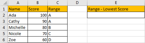
Table of Contents
1. Look Up the Lowest Value by VLOOKUP Function
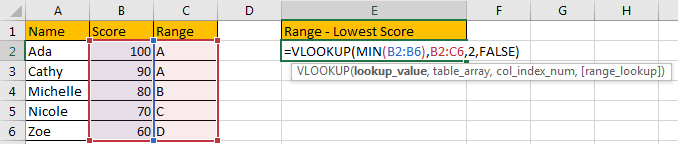
Step1: In E2, enter the formula:
=VLOOKUP(MIN(B2:B6),B2:C6,2,FALSE)As we want to find the ‘Range’ of the lowest score, we need to look up the lowest score among all score first, so we enter MIN(B2:B6) as lookup_value.
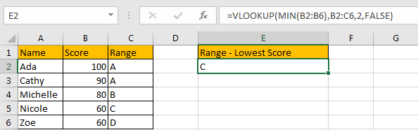
Step2: Click Enter to get returned value in C column.

Comment:
a.If there are two duplicate lowest values, VLOOKUP function will look up the first match value and return its adjacent value.
b.This method only works well when returned value is listed in the right column.
2. Look Up the Lowest Value using User Defined Function with VBA Code
You can also create a User Defined function with VBA Code to lookup the lowest value in a list to replace the above VLOOKUP formula. Just do the following steps:
Step1: Open your Excel workbook and press Alt + F11 to open the Visual Basic Editor.
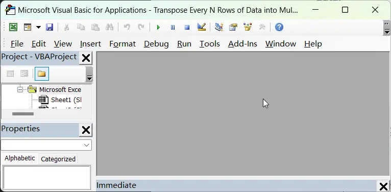
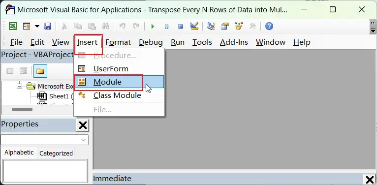
Step2: In the Visual Basic Editor, click Insert > Module to insert a new module.
Step3: Copy the below VBA code for the custom function and paste it into the new module. Save the VBA module by clicking File > Save or by pressing Ctrl + S.
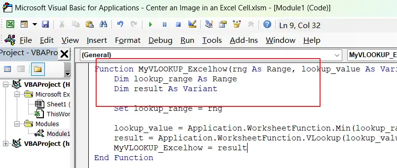
Function MyVLOOKUP_Excelhow(rng As Range, lookup_value As Variant, column_index As Integer, exact_match As Boolean) As Variant
Dim lookup_range As Range
Dim result As Variant
Set lookup_range = rng
lookup_value = Application.WorksheetFunction.Min(lookup_range.Columns(1))
result = Application.WorksheetFunction.VLookup(lookup_value, lookup_range, column_index, exact_match)
MyVLOOKUP_Excelhow = result
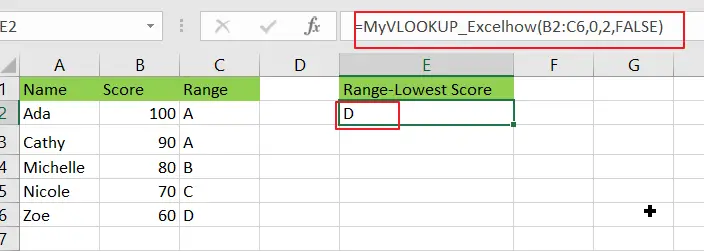
End FunctionStep4: In your Excel worksheet, enter a formula using the custom function just like you would any other built-in Excel function. Enter the following formula in Cell E2:
=MyVLOOKUP_Excelhow(B2:C6,0,2,FALSE)Step5: Press Enter to calculate the result of the formula using the custom function.
3. Look Up the Lowest Value by INDEX/MATCH Functions
In above example, if we want to know the name of the lowest score, VLOOKUP function doesn’t work. So we use INDEX and MATCH functions combination to look up the lowest value here.
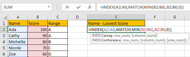
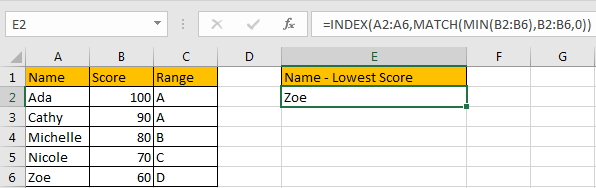
Step1: In B2, enter the formula:
=INDEX(A2:A6,MATCH(MIN(B2:B6),B2:B6,0))MATCH function returns the location of cell, in this example it returns the lowest value’s row number. Then we can use INDEX function to get proper Name from A2:A6 refer to row number.
Step2: Click Enter to get returned value.
Comment:
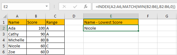
a. If there are two duplicate lowest values, INDEX/MATCH functions will look up the first match value and return its adjacent value.
b. This method works well for that returned value lists on the both sides of match value.
4. Video: Look Up the Lowest Value in A List
This video will demonstrate how to use the VLOOKUP function and VBA code to look up the lowest value in a list in Excel.
5. Related Functions
- Excel INDEX function
The Excel INDEX function returns a value from a table based on the index (row number and column number)The INDEX function is a build-in function in Microsoft Excel and it is categorized as a Lookup and Reference Function.The syntax of the INDEX function is as below:= INDEX (array, row_num,[column_num])… - Excel MAX function
The Excel MAX function returns the largest numeric value from the numbers that you provided. Or returns the largest value in the array.= MAX(num1,[num2,…numn])… - Excel MIN function
The Excel MIN function returns the smallest numeric value from the numbers that you provided. Or returns the smallest value in the array.The MIN function is a build-in function in Microsoft Excel and it is categorized as a Statistical Function.The syntax of the MIN function is as below:= MIN(num1,[num2,…numn])…. - Excel VLOOKUP function
The Excel VLOOKUP function lookup a value in the first column of the table and return the value in the same row based on index_num position.The syntax of the VLOOKUP function is as below:= VLOOKUP (lookup_value, table_array, column_index_num,[range_lookup])…. - Excel MATCH function
The Excel MATCH function search a value in an array and returns the position of that item.The MATCH function is a build-in function in Microsoft Excel and it is categorized as a Lookup and Reference Function.The syntax of the MATCH function is as below:= MATCH (lookup_value, lookup_array, [match_type])….