This post will explain that how to get the maximal or minimal string based on the alphabetic order from a range of cells in Excel. You will learn that how to use the Excel Functions to find or extract the Maximal string or Minimal string based on alphabetic order from a specified range of cells.
Assuming that you have a list of data that contains string values in the range B1:B5.
Table of Contents
Finding Maximal String
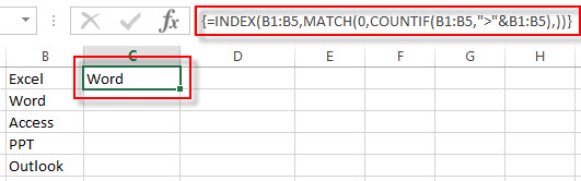
If you want to get the maximal string or largest string based on the alphabetic order, you can use the MATCH function and COUNTIF function to combine with the INDEX function to create the below Excel Array Formula to achieve the result.
{=INDEX(B1:B5,MATCH(0,COUNTIF(B1:B5,">"&B1:B5),)) }
You can enter the above formula into the formula box of Cell C1, then press Ctrl + Shift + Enter shortcuts to change the formula as Array formula. You will see that the maximal string will be extracted.
Let’s see how this formula works:
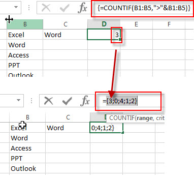
=COUNTIF(B1:B5,”>”&B1:B5)
The COUNTIF function will count the number of cells in range B1:B5 that meet a given criteria. And this criteria is that each value in the range B1:B5 is compared with other values in the same range, and then get the number of text values that is greater than comparing each text value in range B1:B5 with other text values in B1:B5, then counting the number of other text values that is greater than the value.
For example, In range B1:B5, there are 3 text values that is greater than “Excel” text in Cell B1, then the COUNTIF function will return the number 3. To get the number of the other text values based on this criteria, we need to consider to use the array formula. Just see the below screenshot:
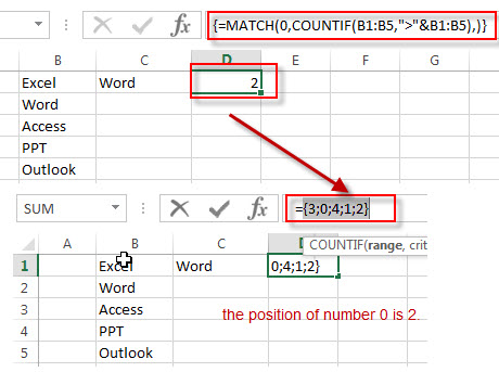
Note: if no any text values are greater than the value, it will return the number 0. And this text value is what we are looking the maximal text value. So we can use this formula combining with the MATCH function to the number 0 in the array list that returned by the COUNTIF function and returns the position of number 0.
{=MATCH(0,COUNTIF(B1:B5,”>”&B1:B5),)}
This function will use the MATCH function to get the position of the number 0, then pass this index value to the INDEX function to get the maximal text value in range B1:B5.
Find Minimal String
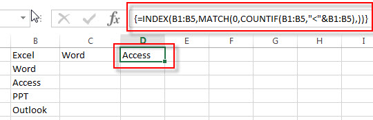
If you just want to find the minimal String, just change the criteria from the above COUNTIF function, so you can write down the following array formula:
{=INDEX(B1:B5,MATCH(0,COUNTIF(B1:B5,"<"&B1:B5),)) }
Related Functions
- Excel INDEX function
The Excel INDEX function returns a value from a table based on the index (row number and column number)The INDEX function is a build-in function in Microsoft Excel and it is categorized as a Lookup and Reference Function.The syntax of the INDEX function is as below:= INDEX (array, row_num,[column_num])… - Excel MATCH function
The Excel MATCH function search a value in an array and returns the position of that item.The syntax of the MATCH function is as below:= MATCH (lookup_value, lookup_array, [match_type])…. - Excel COUNTIF function
The Excel COUNTIF function will count the number of cells in a range that meet a given criteria. This function can be used to count the different kinds of cells with number, date, text values, blank, non-blanks, or containing specific characters.etc.= COUNTIF (range, criteria)…
Leave a Reply
You must be logged in to post a comment.