Assume you have a table consisting of a few cells having few values, and you want to filter out the set of records with the partial match. You might take it easy and would prefer to manually filter out the desired partial matching values into another table without any need for the formula; then congratulations because you are thinking right.
But let me add that it would be a big deal while dealing with a bulk of data in the table, and then doing this bulky task manually would be a foolish decision.
But there isn’t any need to worry about it because after carefully reading this article filtering out the set of records with the aid of partial matches will be a piece of cake for you.
So let’s get straight into it!
Table of Contents
General Formula:
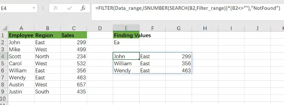
You can use the FILTER function in combination with the SEARCH function to choose data records based on a partial match. The formula in E4 is written as follows:
=FILTER(Data_range,ISNUMBER(SEARCH(B2,Filter_range))*(B2<>""),"Not Found")
Note: Data_range is name range for A2:C9, and Filter_range is antoehr name range for B2:B9.
Let’s See How This Formula Works
The motive is to extract a collection of records that match a partial text string in this example. We match one column in the data range A2:C9 or the “Region” column. The FILTER function (new in Excel 365) retrieves matched data from a range based on a logical filter, which is at the heart of this formula:
=FILTER(filter_data,filter_logic)
The task in this example is to build the logic required to match records based on a partial match. Because the FILTER function does not handle wildcards, we must use an alternative technique. In this situation, we use the SEARCH function in conjunction with the ISNUMBER function as follows:
=ISNUMBER(SEARCH(B2,Filter_range))
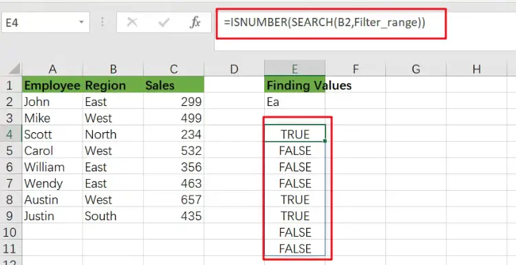
The SEARCH function seeks text input in cell E2 within the Filter_range name range. SEARCH returns the position of a result in the text if it finds one.
If SEARCH formula does not yield any results, it returns the #VALUE! error:
We have a match if SEARCH returns a number. Otherwise, we don’t have a match. We wrap the SEARCH function within the ISNUMBER function to transform this result into a simple TRUE/FALSE value. Only when SEARCH returns a number will ISNUMBER return TRUE.
We aren’t utilizing a wildcard like (“*”) to achieve a partial match, but the SEARCH + ISNUMBER combination acts similarly. SEARCH function will return a number if the search string is found anywhere in the text, and ISNUMBER will return TRUE if the search string is found anywhere in the text.
=FILTER(Data_range,ISNUMBER(SEARCH(B2,Filter_range)))
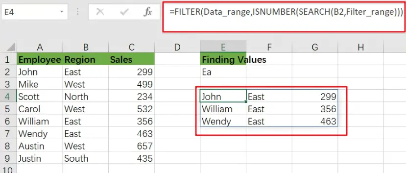
We now have a workable formula, but we still need to clean up a few things. First, if the FILTER function returns no results, it will produce a #CALC! error. We would add a text message for the “if_empty” argument to deliver a friendlier message:
=FILTER(Data_range,ISNUMBER(SEARCH(B2,Filter_range))*(B2<>""),"Not Found")
FILTER will now return “Not Found ” if the search text is not found.
Finally, we must deal with the circumstance where the search string in E2 is blank. Surprisingly, if the search text is an empty string, the SEARCH function will return the value 1.
If field B2 is empty, FILTER will return all results since ISNUMBER will joyfully return TRUE for number 1. To avoid this behavior, we add the following logic to the original logical expression:
=ISNUMBER(SEARCH(B2,Filter_range))*(B2<>"")
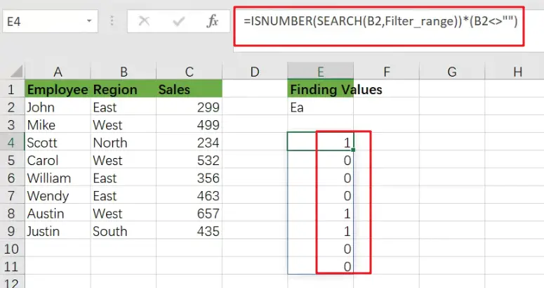
When B2 is not empty, the expression B2<>”” yields TRUE; otherwise, it returns FALSE. By the original SEARCH + ISNUMBER expression, when we would multiply the results of this expression, all TRUE results are “canceled out” when B2 is empty. This is a variation on Boolean logic.
Extract All Partial Match Using Index and Match function
Only Excel 365 supports the FILTER feature. It is feasible to put up a partial match formula in previous versions of Excel to produce more than one match, but it is more complicated. This following formula demonstrates one method based on INDEX and MATCH.
=INDEX($B$1:$B$5,AGGREGATE(15,6,(ROW($B$1:$B$5)-ROW($B$1)+1)/ISNUMBER(SEARCH($D$1,$B$1:$B$5)),E2))
Related Functions
- Excel INDEX function
The Excel INDEX function returns a value from a table based on the index (row number and column number)The INDEX function is a build-in function in Microsoft Excel and it is categorized as a Lookup and Reference Function.The syntax of the INDEX function is as below:= INDEX (array, row_num,[column_num])… - Excel ROW function
The Excel ROW function returns the row number of a cell reference.The ROW function is a build-in function in Microsoft Excel and it is categorized as a Lookup and Reference Function.The syntax of the ROW function is as below:= ROW ([reference])…. - Excel SMALL function
The Excel SMALL function returns the smallest numeric value from the numbers that you provided. Or returns the smallest value in the array.The syntax of the SMALL function is as below:=SMALL(array,nth) … - Excel IF function
The Excel IF function perform a logical test to return one value if the condition is TRUE and return another value if the condition is FALSE. The IF function is a build-in function in Microsoft Excel and it is categorized as a Logical Function.The syntax of the IF function is as below:= IF (condition, [true_value], [false_value])…. - Excel ISNUMBER function
The Excel ISNUMBER function returns TRUE if the value in a cell is a numeric value, otherwise it will return FALSE.The syntax of the ISNUMBER function is as below:= ISNUMBER (value)… - Excel SEARCH function
The Excel SEARCH function returns the number of the starting location of a substring in a text string.The syntax of the SEARCH function is as below:= SEARCH (find_text, within_text,[start_num])… - Excel AGGREGATE function
The Excel AGGREGATE function returns an aggregate in a list or database and ignore errors or hidden rows. The syntax of the AGGREGATE function is as below:= AGGREGATE(function_num, options, ref1,[ref2])… - Excel Filter function
The FILTER function extracts matched records from a collection of data using one or more logical checks. The include argument specifies logical tests, which might encompass a wide variety of formula conditions.==FILTER(array,include,[if empty])…