This post will guide you how to use Excel AGGREGATE function with syntax and examples in Microsoft excel.

Description

The Excel AGGREGATE function returns an aggregate in a list or database and ignore errors or hidden rows.it allow you to apply functions such as: SUM, COUNT, MAX, MIN, SMALL and etc.

The AGGREGATE function is a build-in function in Microsoft Excel and it is categorized as a Math and Trigonometry Function.

The AGGREGATE function is available in Excel 2016, Excel 2013, Excel 2010, Excel 2007, Excel 2003, Excel XP, Excel 2000, Excel 2011 for Mac.

Syntax

The syntax of the AGGREGATE function is as below:

= AGGREGATE(function_num, options, ref1,[ref2])

Where the AGGREGATE function arguments are:
function_num – This is a required argument. The function that you want to use and it can be any of the below number(1-19).

1	AVERAGE
2	COUNT
3	COUNTA
4	MAX
5	MIN
6	PRODUCT
7	STDEV.S
8	STDEV.P
9	SUM
10	VAR.S
11	VAR.P
12	MEDIAN
13	MODE.SNGL
14	LARGE
15	SMALL
16	PERCENTILE.INC
17	QUARTILE.INC
18	PERCENTILE.EXC
19	QUARTILE.EXC

Options – This is a required argument.  A numeric value that determines which values to ignore. If the options is omitted,  the options value will be set to 0.

Value	Explanation
0	Ignore nested SUBTOTAL and AGGREGATE functions
1	Ignore nested SUBTOTAL, AGGREGATE functions, and hidden rows
2	Ignore nested SUBTOTAL, AGGREGATE functions, and error values
3	Ignore nested SUBTOTAL, AGGREGATE functions, hidden rows, and error values
4	Ignore nothing
5	Ignore hidden rows
6	Ignore error values
7	Ignore hidden rows and error values

Ref1 – This is a required argument. The first numeric argument for the functions in aggregate function.
Ref2 – This is an optional argument. Numeric arguments 2 through 253.

Example

The below example will show you how to use Excel AGGREGATE function to return an aggregate in a list.

#1 = AGGREGATE (4,6,B1:B3)

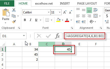
Note: the above formula will calculate the maximum value in the range B1:B3 and ignoring error values.

#2 = AGGREGATE (14,6,B1:B3,2)

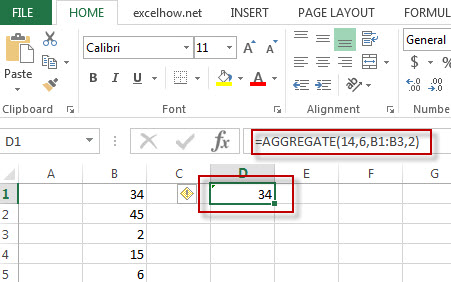
Note: The above excel formula will calculate the second largest value in the range B1:B3 and ignoring error values.