This post will guide you how to extract unique itmes from a given list in Microsoft Excel. How to create a newly formula to get unique values from a range cells in Excel. The unique list of items is the first one found, which does not have a value equal to any other in the array. You can use one formula based on the INDEX function, the MATCH function in combination with the COUNTIF function to extract unique values. The generic formula is as follow:
=INDEX(range, MATCH(0, COUNTIF(unique using, range),0))
Explanation:
This formula will extract unique values from an array or range based on their position rather than just blank cells. First, you need to select the items for your unique list and place them in a range. Then you need to create a new formula in the next blank cell in your worksheet that states, “=INDEX(range, MATCH(0, COUNTIF(unique using, range),0))".
This formula will extract the unique values for just one column. If you prefer to have them in a different column, just drag the formula to that cell. You can also highlight the newly created formula and drag it down throughout your spreadsheet, but be sure to copy the values instead of cutting them before you do so since once you cut or delete them, they are gone.
Lets understand with an example:
"=INDEX($A$1:$A$8,MATCH(0,COUNTIF($C$1:C1,$A$1:$A$8),0))"
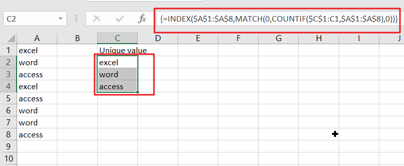
The data in this table consists of the range cells $A$1:$A$8.
To create a formula that automatically sums up all of the values in an array, simply enter Control+Shift+Enter.
Clarification:
This formula starts with a basic index.
=INDEX(range,row)
This is telling Excel to find the row in your list of data where you want to start extracting unique items.
The hard work is figuring out which row number will give us unique values to identify which record needs more attention easily. This process starts with MATCH and COUNTIF; the main trick here is:
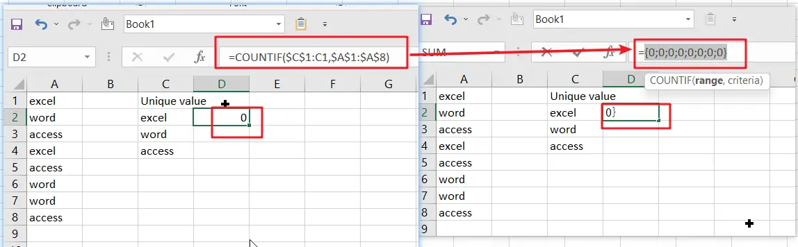
COUNTIF($C$1:C1,range)
With COUNTIF, we can see how many times an item already in our unique list appears on the master list. We use an expanding reference range ($C$1:C1) for this calculation, which means that it will return all values up until but not including $C$.
A growing reference is absolute on one side but relative when copied down. In this case, as the formula gets pasted into each new row of unique data in a list or table structure, it will continue expanding its reach until all available fields have been added with corresponding reference pointing.
To avoid creating a circular reference, we start one row C1 above, where the first unique entry is found. This means we want to count items *already* within that particular list and not just include the current cell. So instead, we begin on the highest able column available at the start.
All the headings should be unique, so they don’t show up in your master list too!
The criteria in COUNTIF returns an array when given multiple values. Therefore, each new row contains different results like this:
{0;0;0;0;0;0;0;0} // row 2
{1;0;0;1;0;0;0;0}// row 3
{1;1;0;1;0;1;1;0}// row 4
As you can see, the MATCH function is able to identify which value in its array is zero. This means we can match each unique entry with a corresponding single-digit number and get all the desired data within our index formula.
The arrays we created in countif can be used to find positions (row numbers). For this, we use MATCH and set it up with an exact match. When put together our two sets produce a result like this:
MATCH(0,{ 0;0;0;0;0;0;0;0},0) // 1 (excel)

MATCH(0,{ 1;0;0;1;0;0;0;0},0) // 2 (word)

MATCH(0,{ 1;1;0;1;0;1;1;0},0) // 3 (access)
The MATCH locator counts items by looking for a count of zero (i.e., when there are no duplicates). This works because it always returns the first match, regardless if others have been found before yours.
INDEX is the key to finding what you’re looking for. It’s like a search engine that returns information by number rather than a name. With this simple difference in methodology comes huge benefits when quickly indexing large volumes of data.
Non-Array Version With LOOKUP
If you are using Excel 2021, you don’t have the INDEX function, but you do have LOOKUP. Lookup can accomplish most of what index can do, except it does it in a linear fashion. It is slow and requires you to enter one value at a time or copy/paste from an adjacent cell range to build your lookup table.
With this formula, you’ll be able to extract all unique items from any list in Excel:
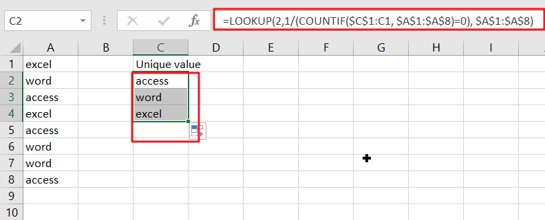
=LOOKUP(2,1/(COUNTIF($C$1:C1, $A$1:$A$8)=0), $A$1:$A$8)
The array operation can be done natively in LOOKUP by using a similar formula as INDEX MATCH.
- Using this, you can simply fill in your list of unique items by using lookup’s maximum row parameter.
- The COUNTIF function returns each value that occurs in the list. The result of COUNTIF is put in a Boolean array [0;1], which yields the count from each item.
- Then divide each number by its own array, creating an even more precise error count.
- When applied as an input to the LOOKUP function, this vector becomes the lookup table that stores all possible values for you!
- The average value of 2 in this lookup_vector is larger than any other value.
- LOOKUP always finds the last non-error value in an array.
- When a value is found in LOOKUP, it returns that value. The range cells will contain all values returned by lookup when there is more than one occurrence of an input variable.”
This blog post discussed how to extract unique items from a list in Excel. We hope these tips will save you time and make it easy for you to get the most important data. If there are any other tricks or shortcuts we can provide, please let us know!
Related Functions
- Excel INDEX function
The Excel INDEX function returns a value from a table based on the index (row number and column number)The INDEX function is a build-in function in Microsoft Excel and it is categorized as a Lookup and Reference Function.The syntax of the INDEX function is as below:= INDEX (array, row_num,[column_num])… - Excel MATCH function
The Excel MATCH function search a value in an array and returns the position of that item.The MATCH function is a build-in function in Microsoft Excel and it is categorized as a Lookup and Reference Function.The syntax of the MATCH function is as below:= MATCH (lookup_value, lookup_array, [match_type])…. - Excel COUNTIF function
The Excel COUNTIF function will count the number of cells in a range that meet a given criteria. This function can be used to count the different kinds of cells with number, date, text values, blank, non-blanks, or containing specific characters.etc.= COUNTIF (range, criteria)… - Excel LOOKUP function
The Excel LOOKUP function will search a value in a vector or array.The syntax of the LOOKUP function is as below:= LOOKUP (lookup_value, lookup_vector, [result_vector])…