This post will show you how to use the most of main features of the conditional formatting in Excel. You can also learn how to do conditional formatting for a selected range of cells or a pivot table in any versions of Excel. How to use preset rules to format text, number or date values, and how to create a newly conditional formatting rule to highlight cells, or how to copy, delete, clear conditional formatting rules in Excel 2013,2016,2019,365.

If you want to apply different formats to the range of cells or pivot table that matches the given conditions, you can use the Conditional Formatting to do it in the Microsoft Excel Spreadsheet. It can spot variances by highlighting specific cells at a very fast rate.

It may seem a little complicated to use conditional formatting for some newly users. Once you have finished reading the below most of contents in this tutorial, you should be pleasantly surprised to discover that Excel Conditional Formatting is actually a breeze to understand and effortlessly implement.

1. What is Conditional Formatting in Excel?

Conditional Formatting in Excel is like having your own personal data stylist. It’s a nifty feature that automatically dresses up your cells based on specific rules or conditions. Just imagine having a clever assistant who can pick out important trends, outliers, or exceptions in your data and highlight them with visual way. It enables you to highlight or format your data in various style by changing cell’s background color, font style, font size, etc.

Assuming that you’re dealing with a massive dataset that holds sales data for various regions. You can create some rules that make certain cells stand out with conditional formatting. For instance, you could make cells with sales exceeding a particular threshold appear in bold font and sport a vibrant green background.

2. How to Find Conditional Formatting in Excel

For most Excel versions (Excel 2013, Excel 2016, Excel 2019, Excel 365), you can locate the Conditional Formatting command by following the steps below.

Step1: just open your Microsoft Excel Application and then try to navigate to the ribbon at the top of the current worksheet.

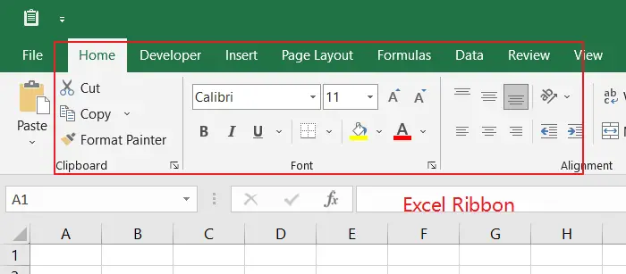
Step2: Look for the Home tab—it’s like the hub of Excel’s essential tools.

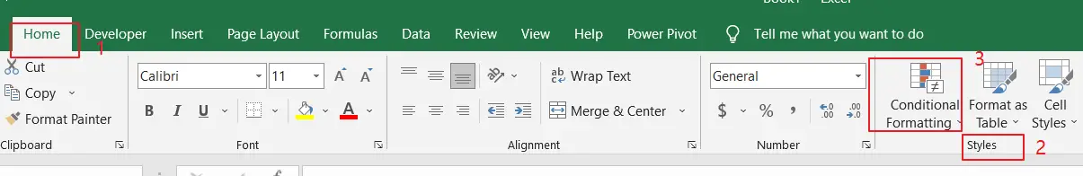
Step3: Once you’re there, keep your eyes searching for a section called Styles.

step4: Within the Styles section, you’ll find a small, inconspicuous button with an enchanting name: Conditional Formatting :). Give it a click, a menu will appear before you.

Now you should know where to find the Conditional Formatting in the most popular version of Excel. Next, you can define the conditions or rules that trigger the formatting.

3. Format or Highlight Cells That Contain Text Values

To more easily find cells that contain the specified text, you can highlight or format them with conditional formatting or preset rules. Just do the following detailed steps.

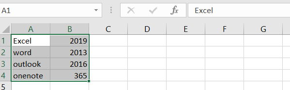
Step1: open your worksheet that contains the cells you want to format (such as: Sheet1).

Step2: select cells where you want to apply the formatting. such as: select A1:B4.

Step3: go to Home in the Excel Ribbon.

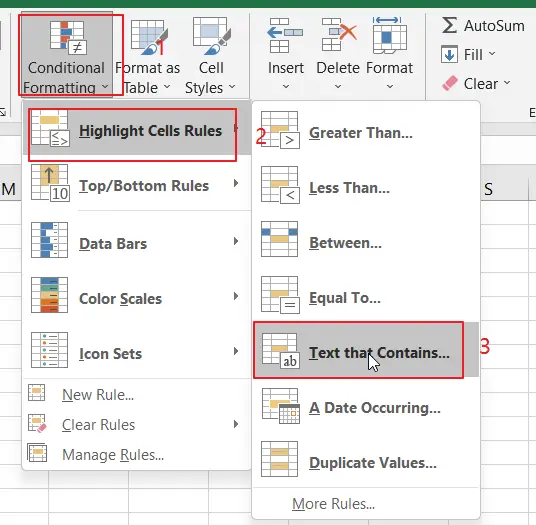
Step4: clicking on Conditional Formatting command under Styles group. a drop-down menu list will open.

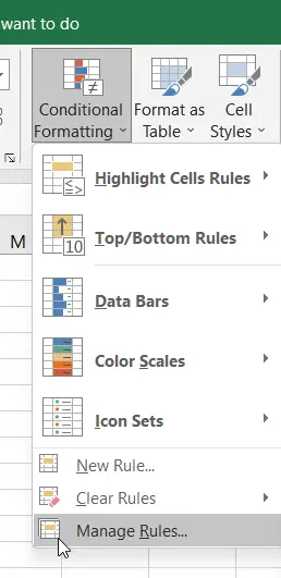
Step5: hover your mouse cursor over the Highlight Cells Rules option in the drop-down menu list. A sub-menu list will open with various highlighting options.

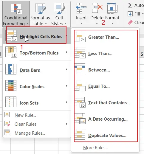
Step6: click on the Text that Contains menu. A dialog box named Text That Contains will pop up, allowing you to specify the text criteria for formatting.

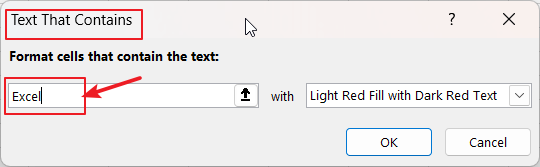
Step7: type one text string or phrase in the first text box in the Text That Contains dialog box. You can type it directly or reference a cell containing the text value. Type “Excel” in this example.

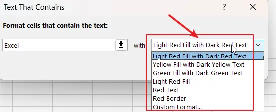
Step8: choose one desired formatting style by selecting a formatting option from the drop-down list. Choose one to highlight the cells with a specific font color, fill color, or both. This example I will select Light Red Fill with Dark Red Text option.

Step9: clicking OK button. It should apply formatting to highlight cells that containing specified text successfully.

Congratulations! You have formatted or highlighted a cell containing a text value successfully in Excel.  Now you can easily spot and focus on those formatted or highlighted cells in your active worksheet.

If you would like to watch videos of the above techniques, just see Video: Format or Highlight Cells That Contain Text Values

4. Format or Highlight Cells That Contain Number Values

To format or highlight cells that contain number values using preset rules in conditional formatting, you can follow these steps:

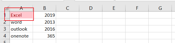
Step1: select one or more cells in a range or table where you want to apply the formats. Select cells B1: B4 in this example.

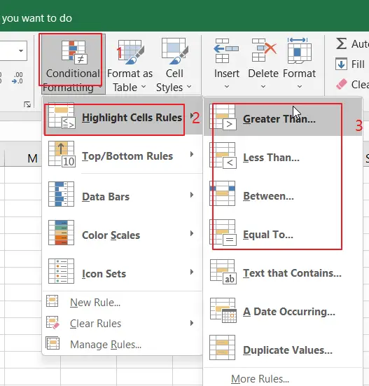
Step2: go to Home tab on the Excel ribbon. Click on Conditional Formatting command under Styles group.

Step3: hover over the Highlight Cell Rules option. Then select one of preset rules based on your requirements in the submenu pop-up list.

Here are some preset rules for conditional formatting feature:

• Greater Than or Less Than: select these options to format cells that are greater than or less than a specified value.
• Between: select this option to format cells that fall within a specific range.
• Equal To: select these two options to format cells that are equal to or not equal to a specific value.

Step4: once you have selected the desired rule and entered the required values (such as: 2017), choose one formatting style you prefer (such as: Green Fill with Dark Green Text) . It contains font color, background color, borders, etc. Just choosing any formatting option that meet your needs.

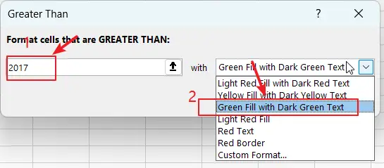
Step5: click OK button to apply the above preset rule that you choosing.

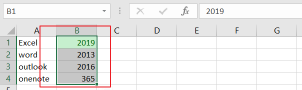
Step6: the selected cells in the range will now be formatted or highlighted based on the preset rule you chose.

See Video: Format or Highlight Cells that contain number values

5. Format or Highlight Cells That Contain Date Values

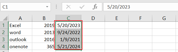
Step1: select range of cells you want to format or highlight in your current worksheet, such as: C1:C4.

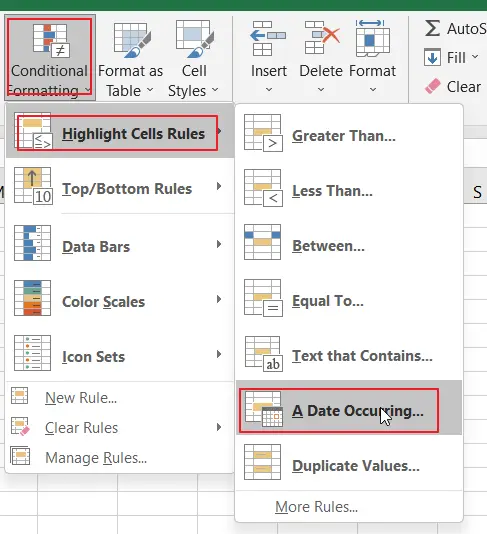
Step2: go to Home tab in the Excel ribbon. click on Conditional Formatting command under Styles group.

Step3: hover over the Highlight Cells Rules option from the drop-down menu list, and another sub menu list will appear.

Step4: select A Date Occurring from the sub menu list. The A Date Occurring dialog box will appear.

Step5: you can select a date comparison, for example, select This Month or Last week as condition, and select one formats from the formatting list, such as: Light Red Fill with Dark Red Text.

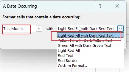
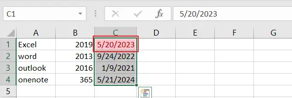
Step6: click OK to apply the preset rule of conditional formatting. The cells that meet the specified conditions will now be formatted according to your chosen formatting style.     

• See Also Video: Format or Highlight Cells That Contain Date Values

6. Format or Highlight Only Unique or Duplicate Values

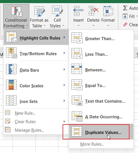
Step1: follow Steps 1-3 mentioned above.

Step2: select Duplicate Values from the Highlight Cells Rules submenu. The Duplicate Values dialog box will open.

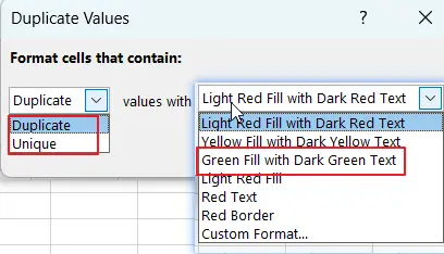
Step3: you can choose Duplicate or Unique as you need in the Duplicate Values dialog box.

Step4: select one formatting style for highlighting the duplicate values, such as, choosing Green Fill with Dark Green Text option.

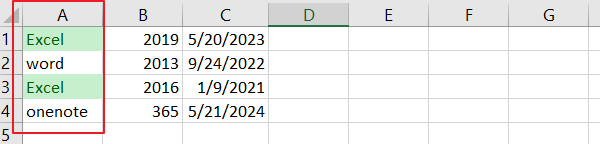
Step5: click OK to apply the conditional formatting. The cells that contain duplicate values within the selected range will now be formatted according to your chosen formatting style.

• See Also Video: Highlight Only Unique or Duplicate Cells

7. Format or Highlight Only Top or Bottom Ranked Values

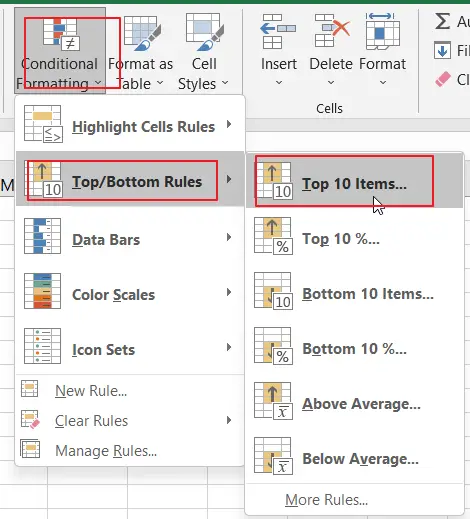
Step1: go to Home tab, then click on Conditional Formatting command under Styles group.

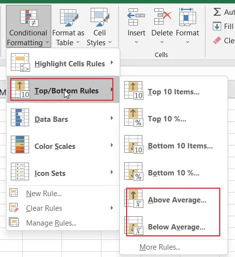
Step2: hover over the Top/Bottom Rules option from the drop-down menu list, and another sub-menu list will appear.

Step3: select one Top or Bottom option from sub menu list, for example, select Top 10 items and the Top 10 items dialog will open.

Step4: type one top-ranked number you want to highlight, for example, set number as 2.

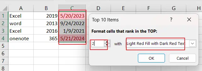
Step5: click OK to apply conditional formatting rule. The cells contain top-ranked values within the selected range will be formatted.

If you would like to watch a video that shows how to highlight only top or bottom 2 values, see Video: Highlight only Top or Bottom Values.

8. Format or Highlight Only Values That are above or below Average

To format or highlight only values that are above or below average values in a range of cells or a pivot table in Excel, you can do the following steps:

Step1: select one or more cells in a range.

Step2: go to Home tab. click on Conditional Formatting command under Styles group.

Step3: clicking on Top/Bottom Rules from the drop-down menu list.

Step4: select one command Above Average or Below Average.

Step5: then select a formatting style, for example, choose Green Fill with Dark Green Text option.

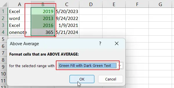
Step6: click OK button. You should see that the selected range contain above or below average values would be formatted based on formats your chosen.

See Also Video: Highlight Only Values That are above or below Average

9. Format or Highlight Cells by Using Data Bars

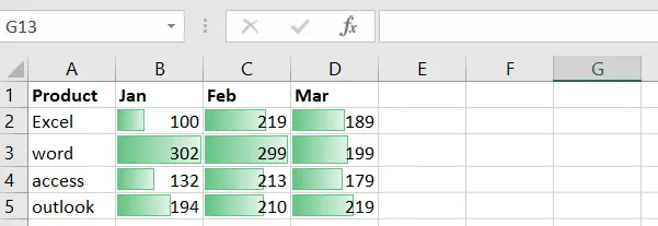
Data bars are a fantastic tool in Excel that brings your data to life! Imagine them as these cool little horizontal bars that magically appear in your cells, giving you a visual representation of your data. It’s like having mini progress bars right in your spreadsheet! These colorful bars not only look pretty, but they also make it easy to compare and analyze your data.

Assuming that you’re working on your worksheet, with a range of cells holding various values. Now, let’s spruce things up! Add data bars, and watch the magic unfold. Each bar’s length corresponds to its cell’s value. Bigger values mean longer bars, while smaller values mean shorter ones. It’s like a visual ranking system, instantly revealing the relative magnitudes of your data.

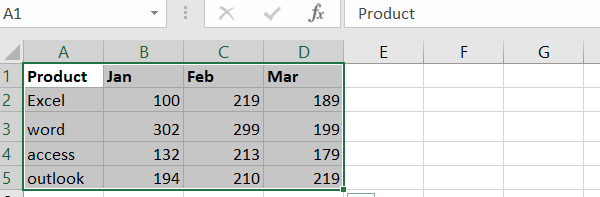
Step1: select cells you want to format, such as, A1:D5.

Step2: go to Home tab in Excel ribbon.

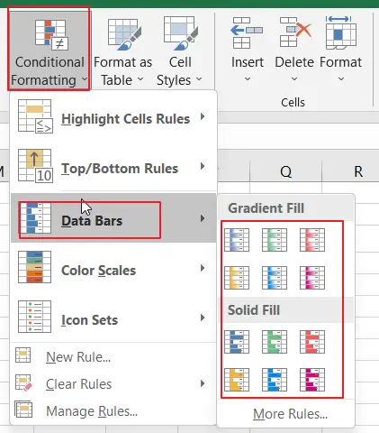
Step3: click on Conditional Formatting button, which is located in Styles group. A dropdown menu will appear.

Step4: select Data Bars from the dropdown menu, another dropdown menu will appear with different options for data bars.

Step5: choose one of the options from the dropdown menu list based on you want the data bars to appear.

Step6: you would see that the selected data bars have been applied to the range of cell you selected.

10. Format or Highlight Cells by Using a Two-color or Three-color Scale

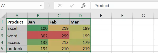
Excel offers two awesome formatting options known as two-color scale and three-color scale. These handy tools use color gradients to visually depict how your data values are interconnected. You can easily identify patterns, trends of your data. It’s like having a reliable visual guide, leading you through ups and downs of your numbers. These formatting settings truly simplify data analysis, making it easy and effortless to understand your data.

Step1: select cells you want to format, such as, A1:D5.

Step2: head over to the Home tab in Excel ribbon.

Step3: click on Conditional Formatting button under Styles group. A dropdown menu list will appear.

Step4: select Color Scales sub-menu from the drop-down list.

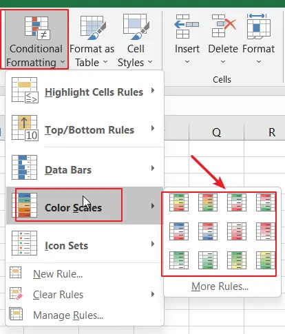
Step5: choose either two-color or three-color scale option based on your preference. You will see that color scale have been applied to cells.

11. Format or Highlight Cells by Using an Icon Set

In Excel’s conditional formatting feature, an icon set is a powerful function that uses symbols to represent data. It’s like a gallery of meaningful icons. Applying it to your data, and Excel will automatically assign icons based on value ranges. This can help you spot trends, patterns, or outliers effortlessly.

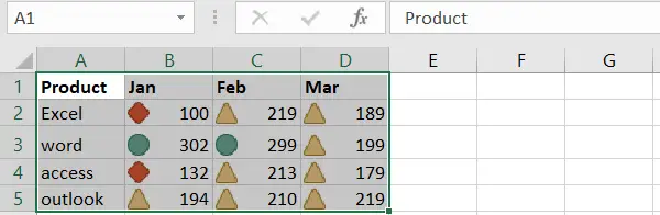
Step1: select cells you want to format, such as, A1:D5.

Step2: head over to the Home tab in the Excel ribbon.

Step3: click on Conditional Formatting button under Styles group. A dropdown menu will appear.

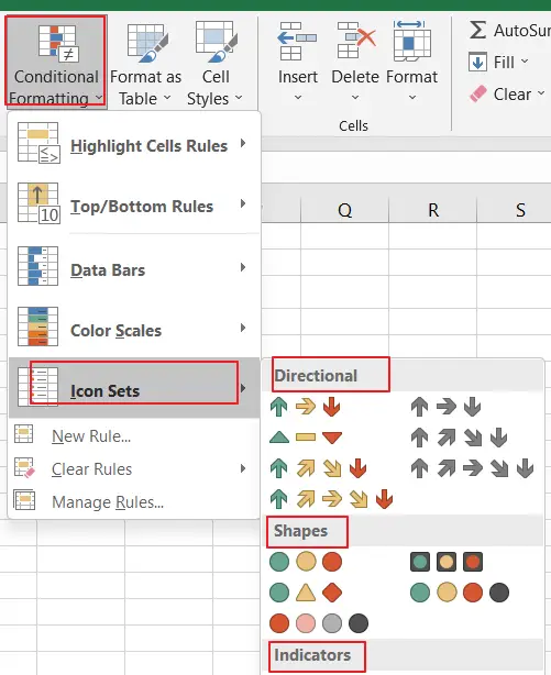
Step4: select Icon Sets sub-menu from the drop-down list.

Step5: you can choose from a collection of icons in different categories, such as: Directional, Shapes, Indicators, or Ratings.

Step6: you would see that icon sets have been applied to the range of cells successfully.

12. Create a Conditional Formatting Rule

You can walk through the steps to create a conditional formatting rule in Excel.

Step1: select cells that you want to apply conditional formatting to, such as, A1:D5.

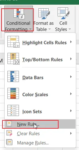
Step2: click Conditional Formatting command under Styles group on the Home tab, a drop-down menu will appear with various formatting options.

Setp3: click New Rule, and New Formatting Rule window will open.

Step4: select one Format Style, such as, 2-Color Scale. click on Ok button.

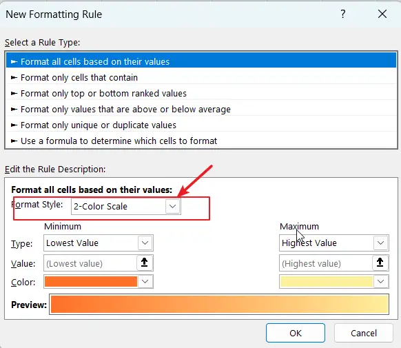
Step5: Excel will immediately apply the conditional formatting rule to the cells, highlighting or formatting them based on the criteria you specified.

See Also Videos: How to Use Conditional Formatting Rule in Excel.

13. Change a Conditional Formatting Rule

You can modify the default rules for conditional formats based on your need.

Step1: open your worksheet that contains conditional formatting rule.

Step2: select cells that have applied conditional formatting rule.

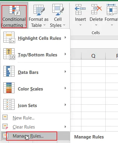
Step3: go to Home tab, click on Conditional Formatting command under Styles group.

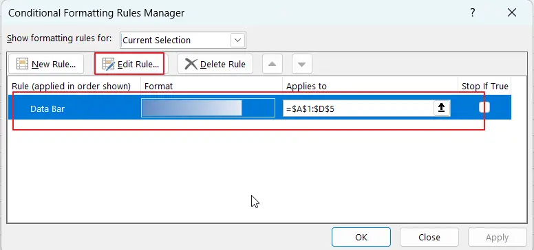
Step4: select Manage Rules from drop down men list. You should see the Conditional Formatting Rules Manager dialog box will open.

Step5: you can see a rule list applied to the selected range of cells. Choose one rule you want to change.

Step6: clicking on Edit Rule button. And you can see the Edit Formatting Rule window will open.

Step7: you can modify some settings based on your requirement, for example, you can try to change Rule Type, adjust Format Style, etc.

Step8: Excel will update conditional formatting rule with new settings.

See Also Videos: How to Use Conditional Formatting Rule in Excel.

14. Apply Multiple Conditional Formatting Rules to Same Cells

You can apply multiple conditional formatting rules to the same cells in Excel. Each rule can have its own criteria and formatting style, for example, you wish to create tree rules to highlight cells, if cell value is greater than 200, then set its background color as red; If cell value is less than 50, set background color as green color; Other cells set background color as yellow.

These rules can be set to work simultaneously, let you analyze different facets of your data in a single view.

15. Copy Conditional Formatting to Another Cell

You can copy conditional formatting to additional cells in Excel. Just do the following steps:

Step1: select the cell that has the conditional formatting that you want to copy.

Step2: go to Home tab, click Format Painter command under Clipboard group, then select cells where you want to copy conditional formatting.

16. Conditional Formatting with Formulas

Excel provide lots of presets that make it easy to create new conditional formatting rules without formulas. If you have some specific conditions that cannot be achieved by presets, at this time, you can use formulas to calculate the difference between values in difference cells as rules and apply formatting based on the result.

Step1: select cells that you want to apply conditional formatting to, such as, A1:D5.

Step2: click Conditional Formatting command under Styles group on the Home tab, a drop-down menu will appear with various formatting options.

Step3: click New Rule, and New Formatting Rule window will open.

Step4: in the New Formatting Rule dialog box that appears, select one type Use a formula to determine which cells to format.

Step5: in the Format values where this formula is true field, enter your formula that will determine the formatting, for example, if you want to highlight cells that contain a value greater than 200, you can enter a formula like: =A1>200 (assuming that Cell A1 is first cell in your selected range).

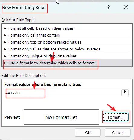
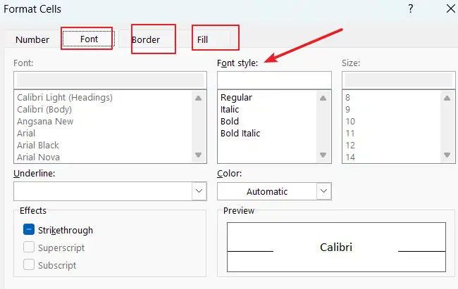
Step6: click on Format button to specify one formatting style you want to apply to cells that meet the condition. You can choose font color, cell background color, borders, etc.

See Also Videos: How to Use Conditional Formatting Rule in Excel.

See Also Other Formulas Examples:

• Highlight Every Other Row Using Conditional Formatting
• Highlight Odd Number and Even Number
• Highlight Cells Based on Their First Letter/Character
• Conditional Format Dates earlier than or Greater Than Today
• Highlight the Dates if its over a year

17. Find Cells That Have Conditional Formatting

If you only want to locate the cells that are formatted in your worksheet, you can do the following steps:

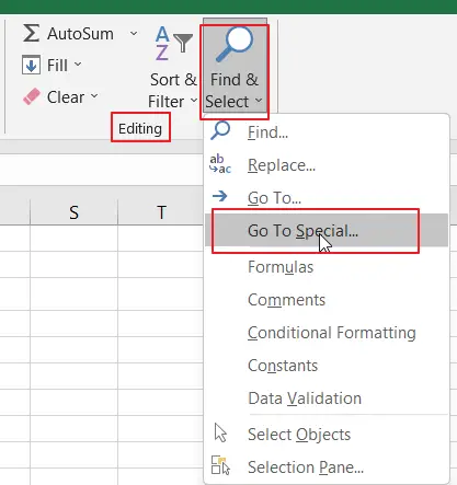
Step1: go to Home tab, click on Find & Select command under Editing group. A drop-down menu list will open.

Step2: select Go To Special sub-menu from the drop-down menu list. A dialog box titled Go To Special will appear.

Step3: select the option Conditional Formats and click on the OK button.

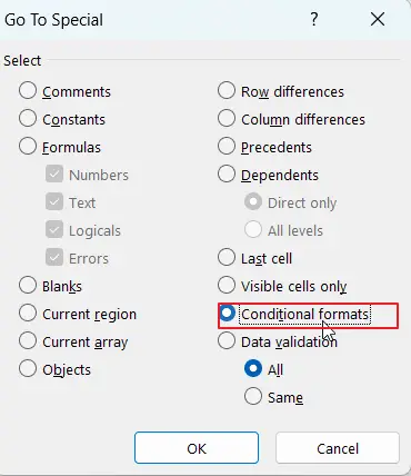
Step4: Excel will now highlight all cells in the worksheet that have conditional formatting applied. You can see the cells being selected or highlighted.

18. Delete a Conditional Formatting Rule

You can delete conditional formats that you do not need in Excel. Just do the following steps:

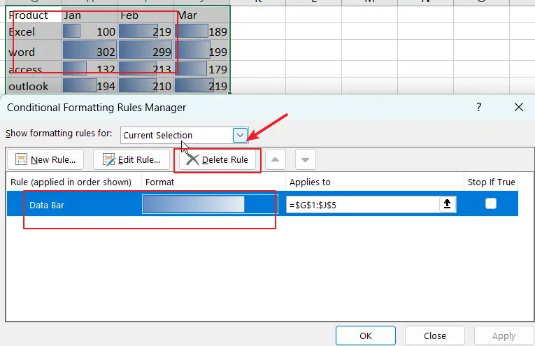
Step1: select one range of cells that contain conditional formatting rule.

Step2: go to Home tab on the Excel Ribbon, and click Conditional formatting command under Styles group.

Step3: click on Manage Rules submenu.

Step4: select the rule that you want to delete, then click Delete Rule button.  Click Ok.

19. Clear Conditional Formatting

If you wish to clear conditional formatting from a selection in Excel, just do the following steps:

Step1: select one range of cells that you want to remove the conditional formatting rules.

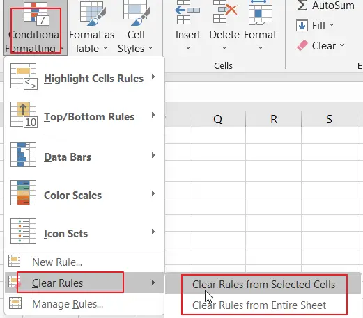
Step2: go to Home tab, click on Conditional formatting command under Styles group, and then select Clear Rules sub menu, click Clear Rules from Selected Cells.

If you want to remove conditional formatting from entire worksheet, just need to click Clear Rules from Entire Sheet.

20. Use Quick Analysis to Apply Conditional Formatting

Step1: when you select one range of cells in worksheet, a small icon named Quick Analysis will appear at the bottom right corner of the selection.

Step2: click on Quick Analysis icon, and a menu will appear with various options.

Step3: in Quick Analysis menu, select Formatting tab. It typically has an icon with a paintbrush.

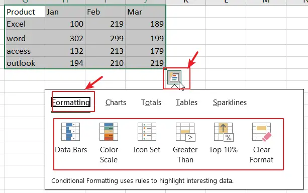
Step4: within the Formatting tab, you’ll see different formatting options such as color scales, data bars, icon sets, and more.