Suppose we have a table of numbers, and we want to highlight odd number and even number by different format settings to distinguish them, in this situation we need to know how to identify odd number and even number. Besides, we need to know how to highlight them by different formats.

Actually, excel has a lot of strong functions, user can highlight odd and even number with different formats by Conditional Format function properly. This article will show you two methods to highlight odd and even number by using Condditional formatting and VBA Code.

1. Identify Odd and Even Number in Excel

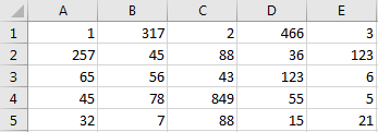
See below table, odd numbers and even numbers exist. We can use ISODD and ISEVEN functions to identify them. See details below.

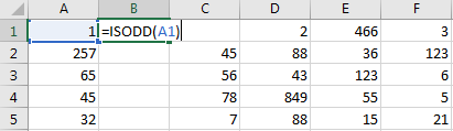
Step1: Insert a new column next to column A. Then in B1, enter the formula =ISODD(A1).

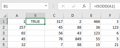
Step2: Click Enter. Verify that True is displayed in B1 properly. That means A1 value is an odd number.

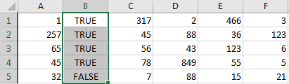
Step3: Drag the fill handler to fill cells B1:B5.

Step4: Select column B, right click and select Copy, then select column D, right click and select Insert Copied Cells.

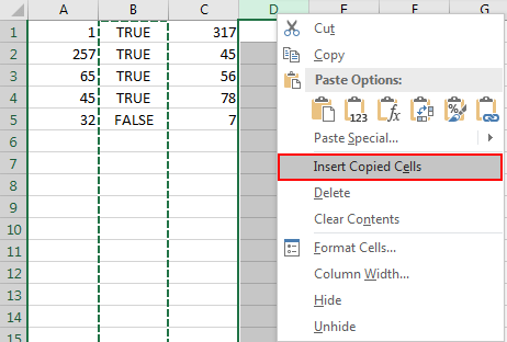
Step5: Then column B with formula will be pasted in D column, True or False value is displayed based on value in column C.

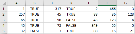
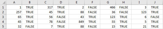
Step6: Repeat above step on other columns. Then you can do filter on column B, D etc. to filter odd number or even number and mark them with different colors.

Note: You can also use ISEVEN function in above steps. This time if value is even number, formula will return True.

2. Highlight Odd and Even Number by Conditional Format in Excel

We can identify odd and even number by above method, though we can do filter on each column and then mark them with different colors, the operation is complex and troublesome. So we need a quick and convenient way to highlight them directly.

We still use previous table to do demonstration.

Step1: First, select the range you want to do filter. In this case select A1:E5.

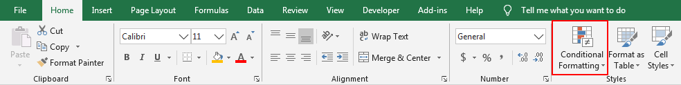
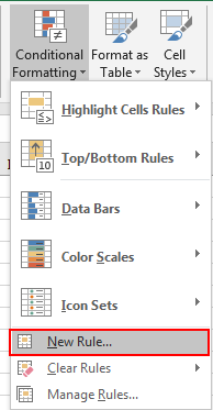
Step2: In ribbon, click Home->Conditional Formatting under Styles.

Step3: Click the arrow button on Conditional Formatting icon to load all sub menus, select New Rule in it.

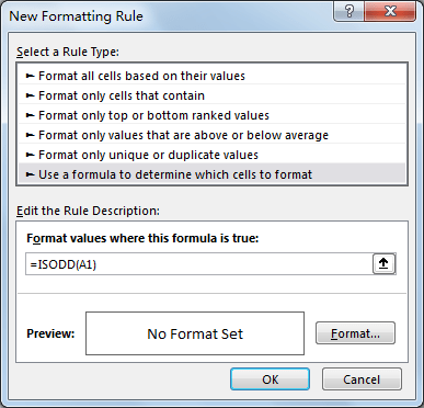
Step4: In the pops up New Formatting Rule window, in Select a Rule Type panel, select Use a formula to determine which cells to format.

Step5: In Edit the Rule Description panel, in Format values where this formula is true textbox, enter the formula =ISODD(A1).

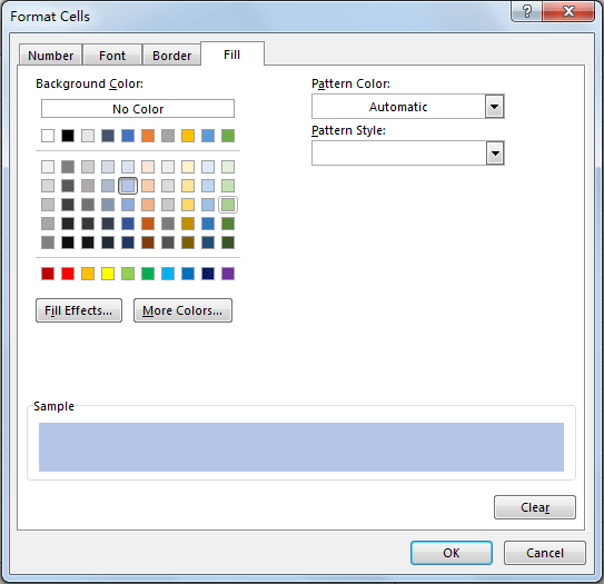
Step6: After entering the formula, click Format button to specify your cell format for highlighted cells. You can design the format by your demands. In this case, we just mark them with light blue background in cells. In Format Cells, click Fill, select Background Color, then click OK.

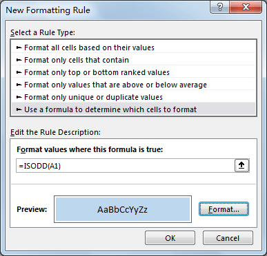
Step7: Returns to New Formatting Rule window, see the Preview. Verify that cell is filled with light blue background. Then click OK.

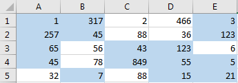
Step8: Verify that all odd numbers are marked with light blue.

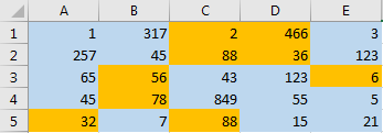
Step9: Repeat above steps, set Format values where this formula is true =ISEVEN(A1), then you can also highlight even numbers with other color.

3. Highlight Odd Number and Even Number with VBA Code

You can also use VBA code to highlight odd and even numbers in the selected range of cells in Excel, just do the following steps:

Step1: Open your workbook that contains the data you want to highlight.

Step2: Press ALT + F11 to open the VBA editor.

Step3: In the VBA editor, go to “Insert” and select “Module“.

Step4: Copy and paste the VBA code into the module. Save the workbook as a macro-enabled workbook (with a .xlsm file extension).

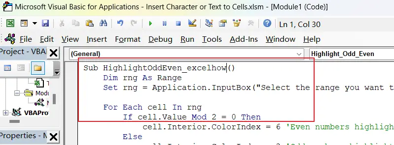
Sub HighlightOddEven_excelhow()
    Dim rng As Range
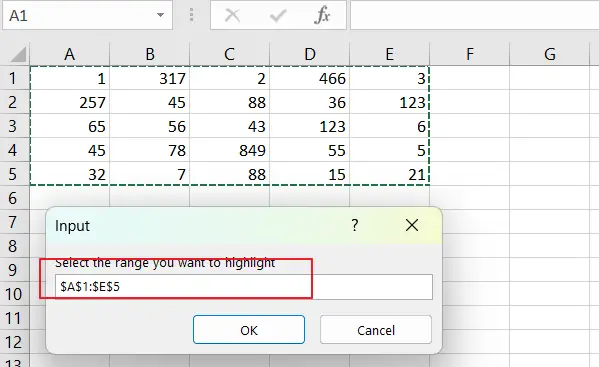
    Set rng = Application.InputBox("Select the range you want to highlight", Type:=8)
    
    For Each cell In rng
        If cell.Value Mod 2 = 0 Then
            cell.Interior.ColorIndex = 6 'Even numbers highlight color (yellow)
        Else
            cell.Interior.ColorIndex = 3 'Odd numbers highlight color (light red)
        End If
    Next cell
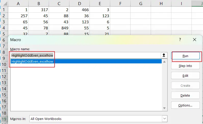
End Sub

Step5: Press ALT + F8 to open the Macro dialog box. Select the macro you want to run. And click “Run“.

Step6: Select the range of cells that you want to highlight.

Step7: The code will loop through each cell in the selected range and highlight even numbers with the color you chose and odd numbers with the other color you chose.

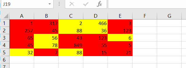
The selected range of cells should now be highlighted based on whether they contain odd or even numbers.

4. Video: Highlight Odd and Even Numbers in Excel

This video will demonstrate how to use conditional formatting and VBA code to highlight odd and even numbers in Excel.