Everybody knows we can easily sort cells by the first character in Excel by Sort feature, but there is no feature or function to sort cells by the last character directly in Microsoft Excel.

This post will guide you how to sort cells by last character in Excel. How do I sort data by the last character with a formula in Excel. How to sort cells based on the last character with User Defined Function in Excel.

1. Sorting Data by Last Character with Formula

Assuming that you have a list of data in range B1:B5, in which contain text string values. And you need to sort cells based on the last characters in cells. We can easily sort cells by the first character, but there is no function or command to sort cells by the last character directly in Microsoft Excel. How to do it. You can use a helper column and then use a formula based on the RIGHT function to extract the last character, then sort helper column, and the column B also be sorted. Here are the steps:

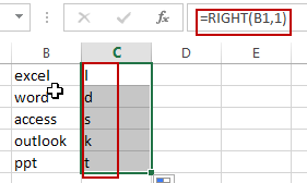
#1 enter the following formula down a nearby column B.

=RIGHT(B1,1)

#2 press Enter key on your keyboard, and then drag the Fill Handle down to other cells.

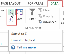
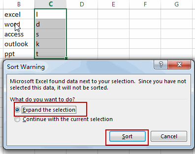
#3 you need to keep selecting the cells in helper column, and go to DATA tab, click Sort A to Z command under Sort & Filter group. Then the Sort Warning dialog will open. Select Expand the selection option in the Sort Warning dialog box. Click Sort button.

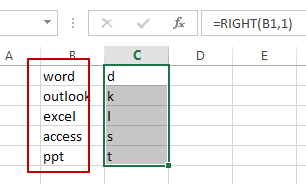
#4 you should notice that the range of cells have been sorted. And now you can delete the helper column.

2. Sorting Data by Last Character with User Defined Function

There is another method to sorting Data by the last character with User Defined Function in Excel. You can try to reverse the text string in Cells, and the last character of original text string will become the first character. So that you can directly sort the cells by the Sort command in the helper column. Here are the steps:

#1 open your excel workbook and then click on “Visual Basic” command under DEVELOPER Tab, or just press “ALT+F11” shortcut.

#2 then the “Visual Basic Editor” window will appear.

#3 click “Insert” ->”Module” to create a new module.

#4 paste the below VBA code into the code window. Then clicking “Save” button.

Public Function ReverseString(R As Range)
    ReverseString = StrReverse(R.Text)
End Function

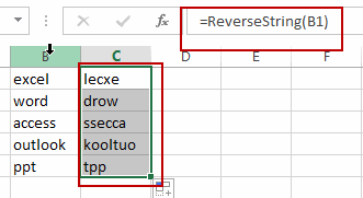
#5 back to the current worksheet, then type the following formula in a blank cell, and then press Enter key.

=ReverseString(B1)

#6 drag the Fill Handle down to other cells.

#7  keep selecting the cells in helper column, and go to DATA tab, click Sort A to Z command under Sort & Filter group. Then the Sort Warning dialog will open. Select Expand the selection option in the Sort Warning dialog box. Click Sort button.

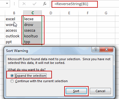
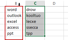
#8 you should notice that the range of cells have been sorted. And now you can delete the helper column.

3. Video: Sort Data by Last Character

This video will guide you how to sort data by the last character with a formula in Excel 2013/2016/2019/365.

4. Related Functions

• Excel RIGHT function
  The Excel RIGHT function returns a substring (a specified number of the characters) from a text string, starting from the rightmost character.The syntax of the RIGHT function is as below:= RIGHT (text,[num_chars])…