This post will guide you how to remove Conditional formatting style in your worksheet in Excel. How do I delete conditional formatting with vba macro in Excel 2013/2016.

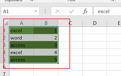
Assuming that you have a list of range which contain product data, and those cells have been highlighted by conditional formatting function. And if there is a easy way to remove conditional formatting quickly in the selected range of cells in your worksheet. This tutorial will show you two methods to remove conditional formatting.

Method1: Remove Conditional Formatting

If you want to remove the conditional formatting quickly in the selected range of cells, and you can do the following steps:

Step 1: select the range of cells that you wish to remove the conditional formatting.

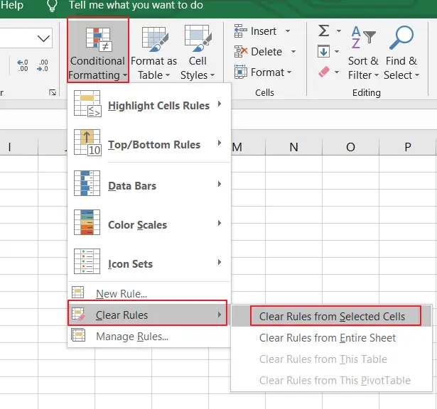
Step 2: go to Home tab, and click Conditional Formatting command under Styles group. select Clear Rules menu from the drop down menu list, and then click on Clear Rules from Selected Cells.

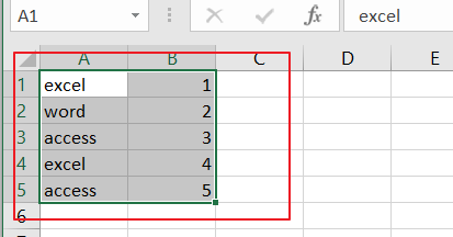
Step 3: you would see that the conditional formatting rules have been removed in the selected range of cells.

Method2: Remove Conditional Formatting with VBA Macro

You can also use an Excel VBA Macro to quickly remove conditional formatting in the selected range of cells. Just do the following steps:

Step1: open your excel workbook and then click on “Visual Basic” command under DEVELOPER Tab, or just press “ALT+F11” shortcut.

Step2: then the “Visual Basic Editor” window will appear.

Step3: click “Insert” ->”Module” to create a new module.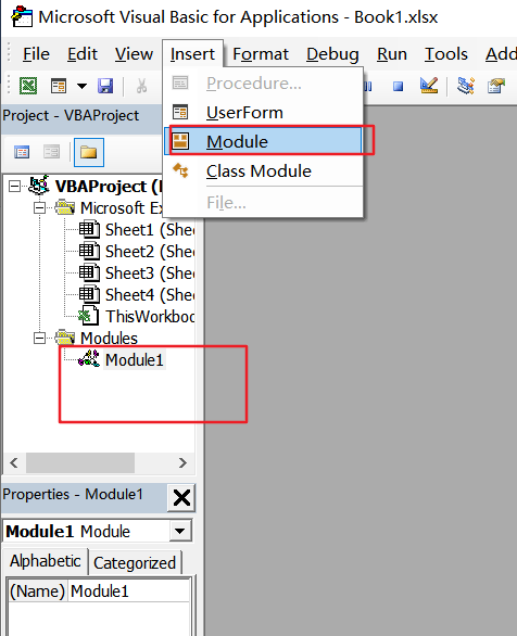

Step4: paste the below VBA code  into the code window. Then clicking “Save” button.

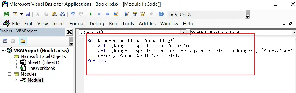
Sub RemoveConditionalFormatting()
    Set myRange = Application.Selection
  Set myRange = Application.InputBox("please select a Range:", "RemoveConditionalFormatting", myRange.Address, Type:=8)
  myRange.FormatConditions.Delete
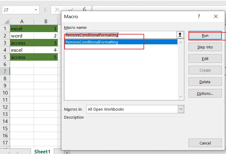
End Sub

Step5: back to the current worksheet, click on Macros button under Code group. then click Run button.

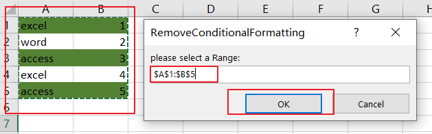
Step6: you need to select one range of cells that you wish to remove conditional formatting, such as: range A1:A5.

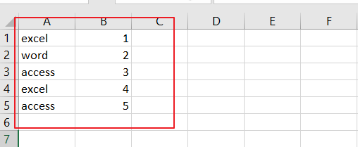
Step7: let’s see the result:

3. Video: Remove Conditional Formatting

This Excel video tutorial, we’ll tackle the task of removing or deleting conditional formatting in Excel using two distinct methods – the ‘Clear Rules’ feature and the power of VBA.