This post will guide you how to highlight cells in which contain formulas using Conditional Formatting feature in Excel. How do I conditionally format a cell if it contains formula using a User defined function in combination with Conditional Formatting feature in Excel 2013/2016.

• Method1: Highlight Cells Containing Formulas Using Defined Name
• Method2: Highlight Cells Containing Formulas Using User Defined Function

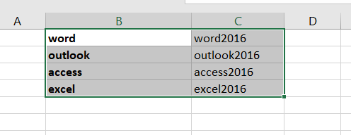
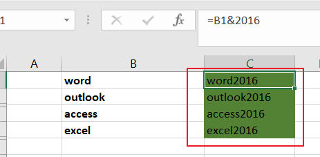
Assuming that you have a list of data in range A1:C5, in which contain product names, sales values and formulas. And you want to only highlight cells if containing formula. How to accomplish it. This post will show you two methods to conditionally format cells if the cells contain formula.

Method1: Highlight Cells Containing Formulas Using Defined Name

---

To highlight Cells containing formulas in your worksheet, you need to create a new range name IsFormula to your workbook. Just do the following steps:

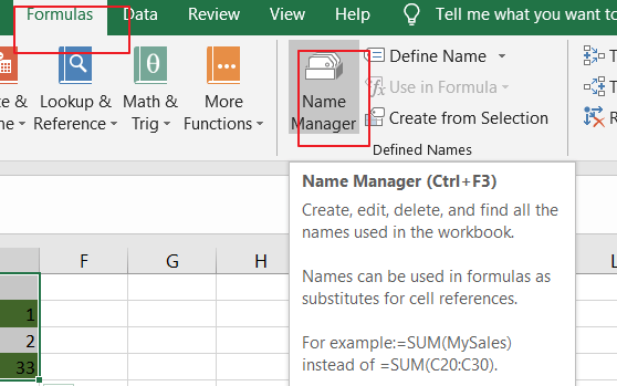
Step1: go to Formulas tab, and click Name Manager button under Defined Names group. and the Name Manager dialog will open.

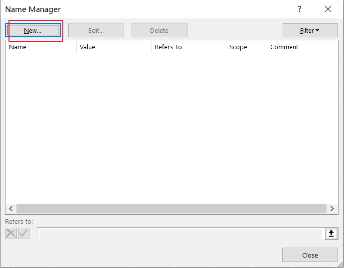
Step2: click New button in the Name Manager dialog box, and the New Name dialog will open.

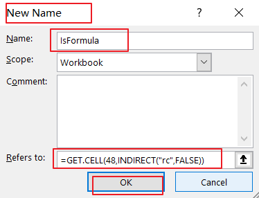
Step3: type a name called IsFormula into the Name text box, and choose Workbook from the drop-down list of Scope. then you need to type the following formula into the Refers to text box. click Ok button.

=GET.CELL(48,INDIRECT(“rc”,FALSE))

Step4: select the range of cells on your worksheet to be conditioanlly formatted for formulas.

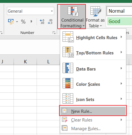
Step5: go to Home tab, click Conditional Formatting command under Styles group, and select New Rule from the drop down menu list. And the New Formatting Rule dialog will open.

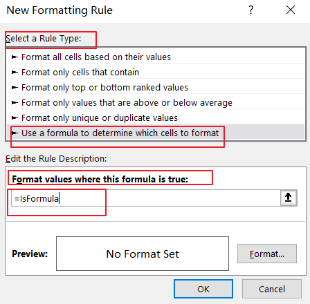
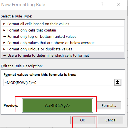
Step6: click Use a formula to determine which cells to format option in the Select a Rule Type section in the New Formatting Rule dialog box, and type the following formula into the Format values where this formula is true text box.

=IsFormula

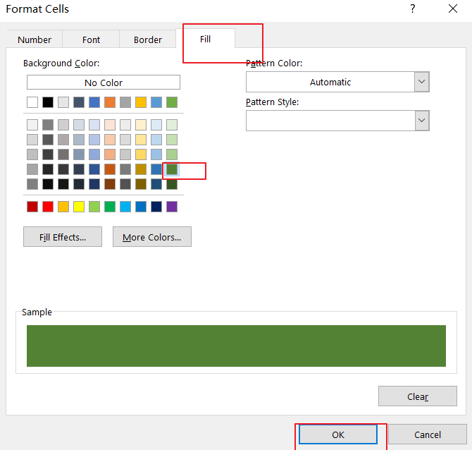
Step7: click Format button, and the Format Cells dialog will open. swith to Fill tab in the Format Cells dialog box, and select one backgroud color as you need to highlight the cells with formulas. click Ok button to back to New Formatting Rule dialog box.

Step8: click OK button, let’ see the last result:

Method2: Highlight Cells Containing Formulas Using User Defined Function

---

You can also use an Excel User Defined Function in conbination with Condtional Formatting feature to highlight cells containing formuals. just do the following steps:

Step1# open your excel workbook and then click on “Visual Basic” command under DEVELOPER Tab, or just press “ALT+F11” shortcut.

Step2#  then the “Visual Basic Editor” window will appear.

Step3# click “Insert” ->”Module” to create a new module.

Step4# paste the below VBA code into the code window. Then clicking “Save” button.

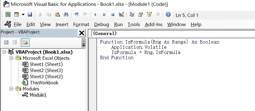
Function IsFormula(Rng As Range) As Boolean
    Application.Volatile
    IsFormula = Rng.IsFormula
End Function

Then you need to repeat the above Step4-Step8 to highlight cells containing formulas in your selected range of cells.