Sometimes we want to highlight some cells based on certain criteria, for example highlight all cells which the first letter is X, this requirement is quite commonly used in searching. Actually, to implement this function, you can highlight these cells by conditional format in excel. This function can help you quickly locate and highlight the cells match your criteria. This article will do a simple introduction about how to highlight cells with the same first letter in their contents by conditional format.
Table of Contents
1. Highlight Cells Based on First Letter/Character by Conditional Format
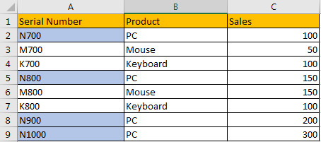
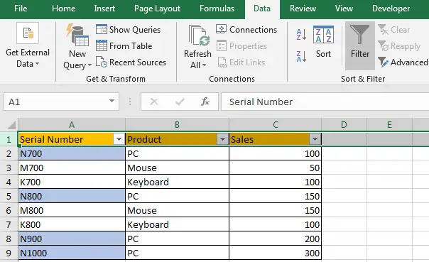
We prepare a list of products for example. They have different serial number. See example below.
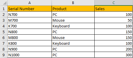
And if we want to check the sales for N or M type of products, we can highlight all cells based on N or M serial number in A column. Now let’s started to learn how can we highlight them by conditional format.
Step1: First, select the range you want to do filter. In this case select A2 to A9.
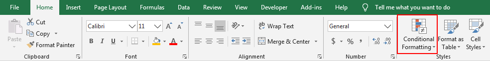
Step2: In ribbon, click Home->Conditional Formatting under Styles.
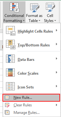
Step3: Click the arrow button on Conditional Formatting icon to load all sub menus, select New Rule in it.
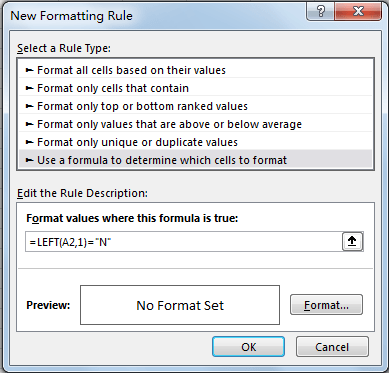
Step4: In the pops up New Formatting Rule window, in Select a Rule Type panel, select Use a formula to determine which cells to format.
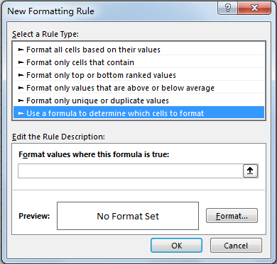
Step5: In Edit the Rule Description panel, in Format values where this formula is true textbox, enter the formula =LEFT(A2,1)=”N”. Notice that if you want to highlight cells with the first number is M, you can change the formula like =LEFT(A2,1)=”M”.
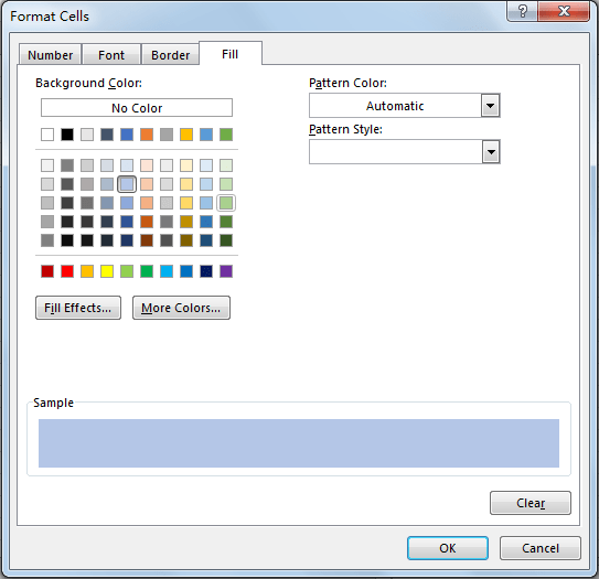
Step6: After entering the formula, click Format button to specify you cell format for highlighted cells. You can design the format by your demands. In this case, we just mark them with light blue background in cells. In Format Cells, click Fill, select Background Color, then click OK.
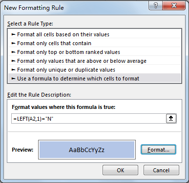
Step7: Returns to New Formatting Rule window, see the Preview. Verify that cell is filled with light blue background. Then click OK.
Step8: Verify that in Serial Number column, cells with N type are highlighted properly.
If you want to only show the rows with N type products, you can follow below steps to filter data.
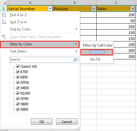
Step9: Select A1 & B1 & C1, click Data->Filter. Then A & B & C columns are added filter.
Step10: Click filter arrow in A column, select Filter by Color, then select background light blue in Filter by Cell Color.
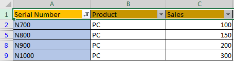
Step11: Verify that only N type products rows are listed.
2. Video: Highlight Cells Based on Their First Letter/Character by Conditional Format in Excel
This video will show you how to use conditional formatting in Excel to highlight cells based on their first letter or character.