This post will guide you how to filter or delete rows with strikethrough format in your selected range of cells in Excel. How do I Filter by strikethrough formatted text with Find and Replace function in Excel 2013/2016. Or how to find cells with strike through formatting in Excel.

1. Filter Data with Strikethrough Formatting Using Find and Replace Feature

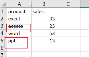
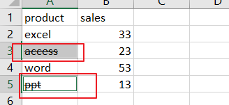
Assuming that you have a list of data in range A1:B5, in which contain data with strikethrough formatting. In other words, those data with strikethrough formatting are useless. And you want to filter all those kinds of cells with strikethrough formatting in your worksheet, then maybe delete it or hide those data, how to do it. This post will show you one method to accomplish it using Find and Replace feature. Just do the following steps:

Step1: select your data in range A1:B5

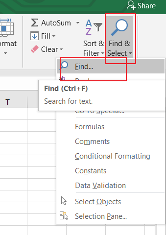
Step2: go to Home tab, click Find & Select button under Editing group. And select Find from the context menu list. And the Find and Replace dialog will open.

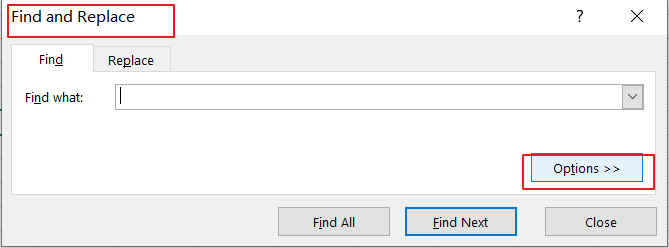
Step3: choose Find tab under the Find and Replace dialog box, and click on Options button.

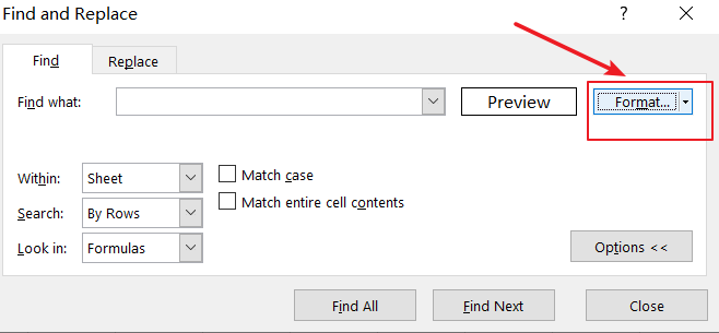
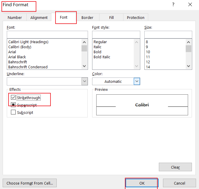
Step4: click on Format button, and select Format…from the popup menu list. And the Find Format dialog will open.

Step5: click on Font tab under the Find Format dialog box, and check Strikethrough checkbox under Effects section. And click Ok button for those above changes to take effect. Now you can see format in the Preview.

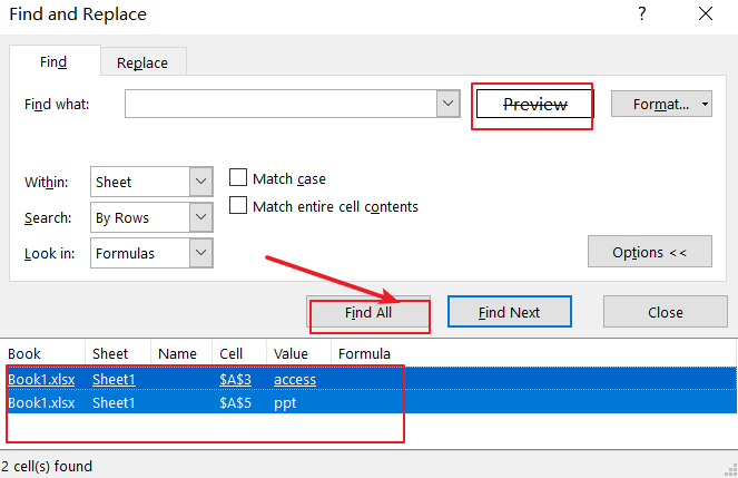
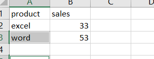
Step6: click Find All button, and the findings are displayed in the below dialog box, then press Ctrl +A keys to select all results. Click Close button. And all cells with Strikethrough are being selected.

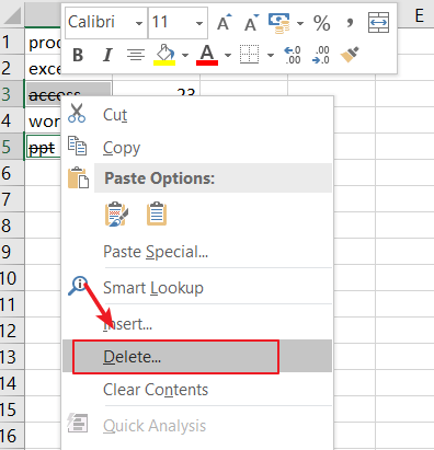
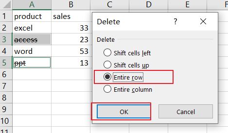
Step7: right click on the selected cells, and select Delete from the context menu. And select Entire row radio button. And click Ok button.

2. Filter Data with Strikethrough Formatting Using User Defined Function

You can also create a macro code module to filter rows by strikethrough formatting in your data. Just do the following steps:

#1 open your excel workbook and then click on “Visual Basic” command under DEVELOPER Tab, or just press “ALT+F11” shortcut.

#2 then the “Visual Basic Editor” window will appear.

#3 click “Insert” ->”Module” to create a new module.

#4 paste the below VBA code into the code window. Then clicking “Save” button.

Function StrikeThrough(R As Range) As Integer
If R.Count = 1 Then StrikeThrough = R.Font.StrikeThrough
End Function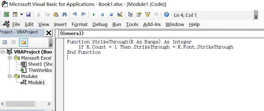

#5 back to the current worksheet, then type the following formula in a blank cell, and then press Enter key. And drag the AutoFill Handle over to other cells.

=StrikeThrough(A1)

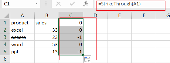
You should see that column C will then flag number 0 or -1 if the cells in column B is struck through and then you can now filter number 0 and -1 in column C with Sort command.

3. Video: Filter Data with Strikethrough Format

This Excel video tutorial where we explore two efficient methods for filtering data with strikethrough format—utilizing “Find and Replace” and employing a VBA macro.