This post will guide you on how to filter cells with bold font formatting in Excel 2013/2016/2019/365 using different methods such as Find and Replace, VBA code.
Filtering cells based on formatting can be very useful when you have a large dataset and want to quickly identify and extract specific data points. We will explore how to use the Find and Replace feature to filter cells with bold font formatting. Additionally, we will show you how to use VBA code to automate this process.
Table of Contents
1. Filter Cells with Bold Font Formatting Using Find and Replace Feature
To filter cells with bold font formatting in Excel using Find and Replace, you can follow these steps:
Step1: Select the range of cells that you want to filter.
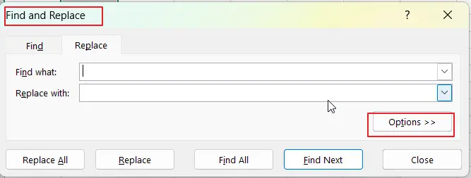
Step2: Press “Ctrl + H” on your keyboard to open the “Find and Replace” dialog box. Click on the “Options” button to expand the options.
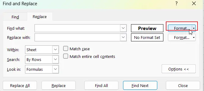
Step3: Click on the “Format” button to open the “Find Format” dialog box.
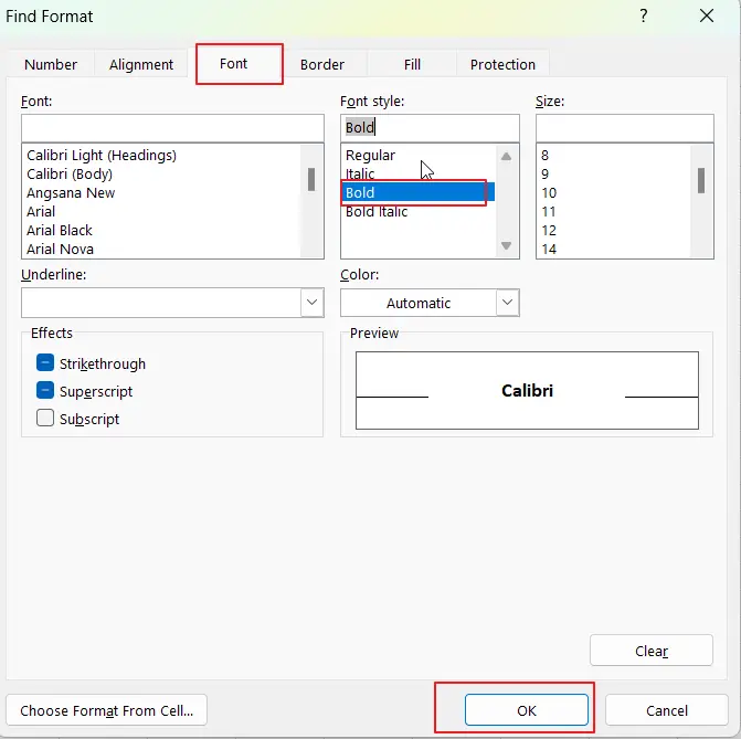
Step4: In the “Find Format” dialog box, switch to Font Tab, select the “Font Style” as “Bold“. Click “OK” to close the “Find Format” dialog box.
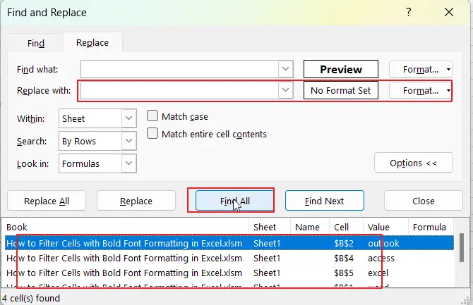
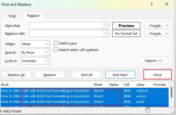
Step5: In the “Find and Replace” dialog box, leave the “Replace with” field empty. Click on the “Find All” button to find all cells with bold font formatting.
Step6: Select all the cells that appear in the search results by pressing “Ctrl + A“. click on Close button.
Step7: Copy the selected cells by pressing “Ctrl + C“. Paste the selected cells into a new worksheet or a new location in the same worksheet.
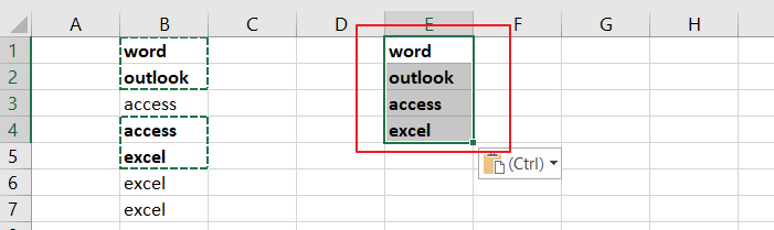
This will filter out all cells without bold font formatting and paste the cells with bold font formatting in a new location for further analysis or manipulation.
2. Filter Cells with Bold Font Formatting with VBA Code
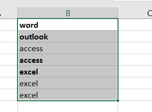
Assuming that you have a list of data in range B1:B5, in which contain text values, and you want to filter those cells with bold font formatting, how to do it. You can use an Excel VBA Macro to accomplish it. Just do the following steps:
Step1: select the range that you want to filter cells with bold font.
Step2: open your excel workbook and then click on “Visual Basic” command under DEVELOPER Tab, or just press “ALT+F11” shortcut.
Step3: then the “Visual Basic Editor” window will appear.
Step4: click “Insert” ->”Module” to create a new module.
Step5: paste the below VBA code into the code window. Then clicking “Save” button.
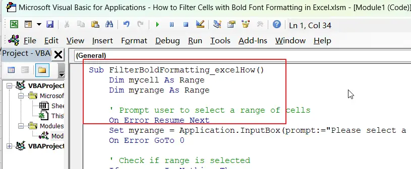
Sub FilterBoldFormatting()
Dim mycell As Range
Dim myrange As Range
' Prompt user to select a range of cells
On Error Resume Next
Set myrange = Application.InputBox(prompt:="Please select a range of cells", Type:=8)
On Error GoTo 0
' Check if range is selected
If myrange Is Nothing Then
MsgBox "No range selected"
Exit Sub
End If
' Loop through each cell in the selected range
For Each mycell In myrange
' Hide the entire row if the cell's font is not bold
If mycell.Font.Bold = False Then
mycell.EntireRow.Hidden = True
End If
Next mycell
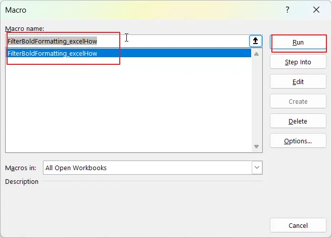
End SubStep6: back to the current worksheet, then run the above excel macro. Click Run button.
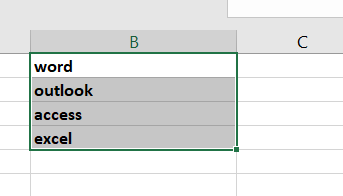
Step7: let’s see the result:
3. Video: Filter Cells with Bold Font Formatting
This video will guide you how tofilter cells with bold font formatting in Excel with different methods.
Leave a Reply
You must be logged in to post a comment.