In our daily work we may need to create a dynamical dropdown list and sort all values by alphabetical order. To create a dropdown list like this, we need to apply some built-in features like ‘Define Name’ and ‘Data Validation’ features, and we also need the help of formula which is combined with excel functions. It sounds complex, but through this tutorial we will introduce you the way to create dynamical dropdown list clearly, we will show you the details by steps, you can follow each step to complete all operations and reach your goal finally.
Precondition:
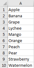
Prepare a list full of different fruits. We may also add new fruits into the list. Now we want to create a dynamical dropdown list and sort fruits by alphabetically order.
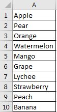
Table of Contents
1. Create Dynamical Drop-Down List and Sort Alphabetically
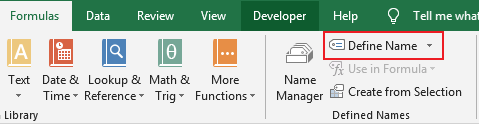
Step 1: Select this fruit list and click Formulas in ribbon, and select Define Name under Defined Names group.
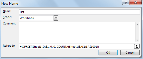
Step 2: In New Name dialog, enter Name as ‘List’, keep Scope unchanged, enter formula =OFFSET(Sheet1!$A$1, 0, 0, COUNTA(Sheet1!$A$1:$A$1001)) into Refers to. Then click OK. Please notice that in this formula ‘Sheet1’ is current sheet name, $A$1 is the first cell of your selected data.
Step 3: Create sheet2, in A1 enter the formula =IF(COUNTA(List)>=ROWS($A$1:A1), INDEX(List, MATCH(SMALL(COUNTIF(List, “<“&List), ROW(A1)), COUNTIF(List, “<“&List), 0)), “”). In this formula, ‘List’ is defined name in last step.

Step 4: As above formula is an array formula, so press Ctrl+Shift+Enter to get value.
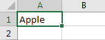
We get the first fruit ‘Apple’ from original table.
Step 5: Drag the fill handle down till blank cell displays.
Note:
If you are confused about above formula and cannot apply it correctly in your work with your instance, you can directly copy the whole list from sheet1 to sheet2, and then sort them by A->Z. Then when you adding new parameters into sheet1 original list, you have to copy this list into sheet2 and sort again.
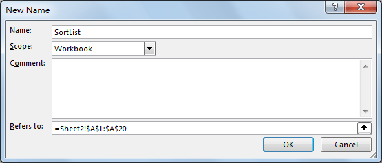
Step 6: Click Formulas in ribbon, and select Define Name under Defined Names group. Enter ‘SortList’ as Name, enter =Sheet2!$A$1:$A$20 into Refers to. Then click OK. Please notice that as we create a dynamically dropdown list, so we can add new parameters into the list without limit, in this instance we set ‘Refer to’ range $A$1:$A$20, so only the first 20 cells in A column can be listed in dropdown list. You can change the reference per your demand.
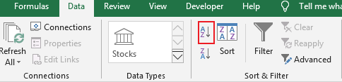
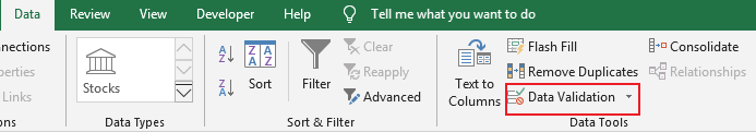
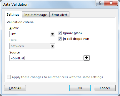
Step 7: Select C2 to locate dropdown list. Click Data->Data Validation under Data Tools group to create data validation.
Step 8: In Data Validation window, under Settings tab, under Allow dropdown list select ‘List’; Enter =SortList in Source. Then click OK.
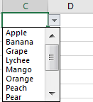
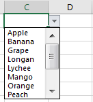
Step 9: Verify that dropdown list is created. Values are sorted by alphabetical order properly.
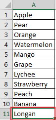
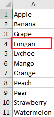
Step 10: Add a new fruit ‘Longan’ into sheet1 original list. You can see that it is added into sheet2 list automatically with proper order, and it is also displayed in dropdown list properly.
Sheet1: Sheet2: Dropdown list:
2. Video: Create Dynamical Drop-Down List and Sort by Alphabetical Order
This Excel video tutorial, we’ll guide you through the process of creating a dynamic drop-down list that automatically sorts values in alphabetical order.
3. Related Functions
- Excel INDEX function
The Excel INDEX function returns a value from a table based on the index (row number and column number)The INDEX function is a build-in function in Microsoft Excel and it is categorized as a Lookup and Reference Function.The syntax of the INDEX function is as below:= INDEX (array, row_num,[column_num])… - Excel MATCH function
The Excel MATCH function search a value in an array and returns the position of that item.The MATCH function is a build-in function in Microsoft Excel and it is categorized as a Lookup and Reference Function.The syntax of the MATCH function is as below:= MATCH (lookup_value, lookup_array, [match_type])…. - Excel IF function
The Excel IF function perform a logical test to return one value if the condition is TRUE and return another value if the condition is FALSE. The IF function is a build-in function in Microsoft Excel and it is categorized as a Logical Function.The syntax of the IF function is as below:= IF (condition, [true_value], [false_value])…. - Excel ROW function
The Excel ROW function returns the row number of a cell reference.The ROW function is a build-in function in Microsoft Excel and it is categorized as a Lookup and Reference Function.The syntax of the ROW function is as below:= ROW ([reference])…. - Excel COUNTA function
The Excel COUNTA function counts the number of cells that are not empty in a range. The syntax of the COUNTA function is as below:= COUNTA(value1, [value2],…)… - Excel COUNTIF function
The Excel COUNTIF function will count the number of cells in a range that meet a given criteria. This function can be used to count the different kinds of cells with number, date, text values, blank, non-blanks, or containing specific characters.etc.= COUNTIF (range, criteria)… - Excel SMALL function
The Excel SMALL function returns the smallest numeric value from the numbers that you provided. Or returns the smallest value in the array.The syntax of the SMALL function is as below:=SMALL(array,nth) …