This post will guide you how to count the number of cells that are not equal to many things in a given range cells using a formula in Excel 2013/2016. You can easily to count cells not equal to a specific value through COUNTIF function. But if there is an easy way to count cells which are not equal to one of many values defined in a selected range of cells in Microsoft Excel. You can count cells that are not equal to many things with a combined formula based on the SUMPRODUCT function, the ISNA function and the MATCH function.

Count Cells not equal to one of many Things

---

Actually, if you just have two or three things that you don’t want to count in your data list, and you can only use one COUNTIFS function like below:

=COUNTIFS(A2:A6,”<>excel”,A2:A6,”<>word”)

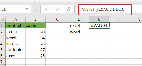
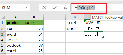
The above formula does not scale very well if you have a list of many things that you do not count, since you have to add more range and criteria pair to for each thing that you do not want to count in range. In this case, you can use the MATCH function to find cells in range A2:A6 that are not equal to values in range D1:D2 like this:

=MATCH(A2:A6,D1:D2,0)

Pressing “Fn” + “F9” or “F9” short key to display the array results like this:

={1;2;#N/A;#N/A;1}

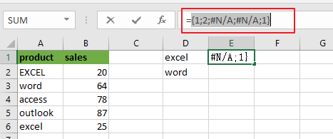
A2:A6 is the lookup value and D1:D2 is the lookup array. Since there are more than one lookup value in range D1:D2, so it returns more than one result in an array result like below:

MATCH function returns the position of lookup values in the lookup array, if lookup value is not in lookup array, it will return #N/A errors. Actually, the numbers of “#N/A” is the number of cells that are not equal to things in D1:D2.

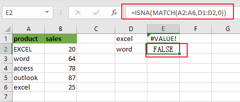
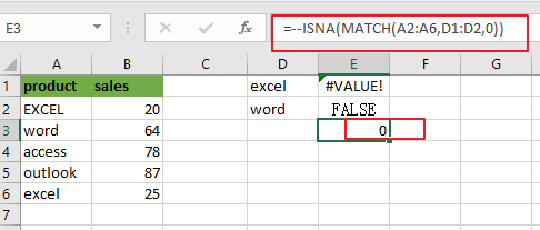
Then you can use the ISNA function to convert all values in the above array result to TRUE or FALSE, like below:

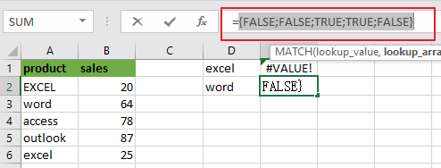
=ISNA(MATCH(A2:A6,D1:D2,0))

={FALSE;FALSE;TRUE;TRUE;FALSE}

Next, you need to use a double negative operator to convert TRUE or FALSE value as 1 or 0 in the above array result. Like below:

=–ISNA(MATCH(A2:A6,D1:D2,0))

={0;0;1;1;0}

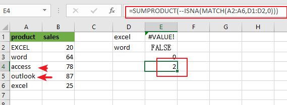
Last, passing the above resulting array to the SUMPRODUCT or SUM function looks like below:

=SUMPRODUCT(–ISNA(MATCH(A2:A6,D1:D2,0)))

Or

{=SUM(–ISNA(MATCH(A2:A6,D1:D2,0)))}

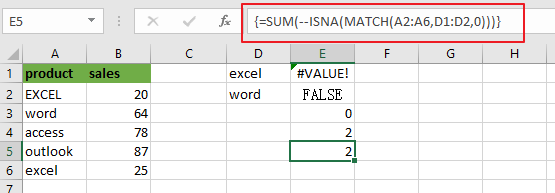
Note: if you are using SUM function in the above formula, you need to press “CTRL + SHIFT + ENTER” shortcuts to convert the formula as a array formula. And the SUMPRMDUCT function can handle the array result by itself.

You can also use another method to count cells which are not equal to many things with a combined formula that utilizes the COUNTA, SUMPRODUCT, and COUNTIF functions.

The general formula is like this:

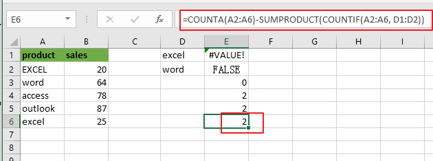
=COUNTA(range)-SUMPRODUCT(COUNTIF(range, things))

In this case, use the following formula:

=COUNTA(A2:A6)-SUMPRODUCT(COUNTIF(A2:A6, D1:D2))

Let’s see how this formula works:

The COUNTA function will count all of the cells in the range A2:A6. And the total number of cell in range A2:A6 is 5.

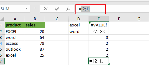
The COUNTIF function will check the range A2:A6 that contain the values in range D1:D2. Then it returns an array result like this:

=COUNTIF(A2:A6, D1:D2)

={2;1}

The SUMPRODUCT function adds up all numbers in the above resulting array, then the returned number is subtracted from the count of all the values in range A2:A6.

The solution logic is that calculating the count of cells that having specific values and then subtract it from the count of all non-empty cells in range A2:A6.

Related Functions

---

• Excel SUMPRODUCT function
  The Excel SUMPRODUCT function multiplies corresponding components in the given one or more arrays or ranges, and returns the sum of those products. The syntax of the SUMPRODUCT function is as below:= SUMPRODUCT (array1,[array2],…)…
• Excel COUNTIF function
  The Excel COUNTIF function will count the number of cells in a range that meet a given criteria. This function can be used to count the different kinds of cells with number, date, text values, blank, non-blanks, or containing specific characters. etc. = COUNTIF (range, criteria) …
• Excel MATCH  function
  The Excel MATCH function search a value in an array and returns the position of that item.The MATCH function is a build-in function in Microsoft Excel and it is categorized as a Lookup and Reference Function.The syntax of the MATCH function is as below:= MATCH  (lookup_value, lookup_array, [match_type])….
• Excel COUNTIFS function
  The Excel COUNTIFS function returns the count of cells in a range that meet one or more criteria. The syntax of the COUNTIFS function is as below:= COUNTIFS(criteria_range1, criteria1, [criteria_range2, criteria2]…)…
• Excel SUM function
  The Excel SUM function will adds all numbers in a range of cells and returns the sum of these values. You can add individual values, cell references or ranges in excel.The syntax of the SUM function is as below:= SUM(number1,[number2],…)
• Excel ISNA function
  The Excel ISNA function used to check if a cell contains the #N/A error, if so, returns TRUE; otherwise, the ISNA function returns FALSE.The syntax of the ISNA function is as below:=ISNA(value)….
• Excel COUNTA function
  The Excel COUNTA function counts the number of cells that are not empty in a range. The syntax of the COUNTA function is as below:= COUNTA(value1, [value2],…)…