In our daily work, we may encounter such an issue that to find the closest value to a certain value. In fact, Excel internal functions can help us solve this problem. In today’s article, we will show you how to find the student whose score value is closet to the score provided with help of Excel INDEX/MATCH/MIN/ABS functions.
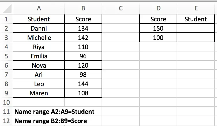
Look at the following example, we want to know who has a score closest to score “150” or “100”.
Expect Result:
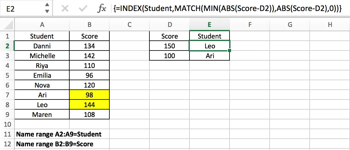
Table of Contents
GENERAL FORMULA
The general formula for this case is
=INDEX(Data,MATCH(MIN(ABS(Data-ProvideValue)),ABS(Data-ProvideValue),0))
In the general formula, you can replace Data and ProvideData with your own range or data reference. This is an array formula and we need to press “control + shift + enter” after entering the formula.
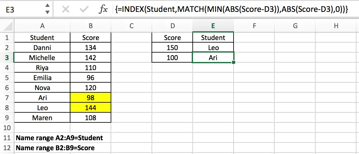
In the above example, the formula is
=INDEX(Student,MATCH(MIN(ABS(Score-D2)),ABS(Score-D2),0)).
In the formula, Data is “Student” list (A2:A9, named “Student”); there are two provided values, 150 in D2 and 100 in D3; In this example, we want to find the closest score to the provided score (in D2 and D3) from the “Scores” list and retrieve the matching student name from the “Students” list that will be returned by the formula and filled in correctly in E2 and E3. Enter above formula in C8, then copy down the formula, the matching students are filled in properly.
Notes:
If we want to only obtain the score value instead of the student, we can just change the lookup array from Student to Score in this formula.
=INDEX(Score,MATCH(MIN(ABS(Score-D2)),ABS(Score-D2),0))
EXPLANATION
For the formula, the core is the usage of Excel INDEX and MATCH functions combination. Before we can explain this formula, we need to know these two functions.
MATCH is an Excel function for locating the position of a query value in a row, column, or table. INDEX is used to return the value at a certain position. As you can see, the MATCH function can provide a relative position of a value within a range, and INDEX can provide a suitable value based on the position provided, so typically, the MATCH and INDEX functions are used together to retrieve a value at a matching position.
Syntax:
=MATCH(lookup_value, lookup_array, [match_type]) (match type 0=exact match)

=INDEX(array, row_num, [column_num])
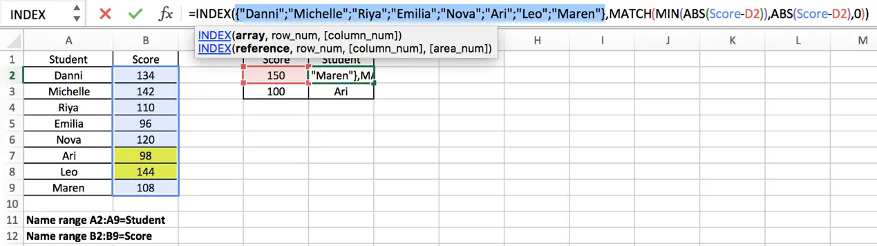
In this example, using E2 as an example, we want to return the name of the student whose score retrieved from the student list is closest to the score 150 provided in D2, so for INDEX function in this formula, the array is the named range “Student” (A2:A9). We expand this array in the formula bar, the array is generated:
{"Danni";"Michelle";"Riya";"Emilia";"Nova";"Ari";"Leo";"Maren"}
In this INDEX function, the parameter “row_number” is obtained by executing another Excel MATCH function. MATCH function will delivery its result to INDEX as row number. The hard work in this case is to find the closest score in Score list to the data provided in D column and obtain the relative position of this score in Score list. To resolve this issue, we use Excel ABS and MIN functions in MATCH expression to obtain the minimum difference between the data and the data provided, and with their help, MATCH function can return the position of the closest score. To let you know how it works step by step, we will explain the expression from inside to outside as the result of the internal function will be delivered to the external one.
First, let’s get to know what the role ABS and MIN functions play in MATCH function.
ABS Function is used to return the absolute value of an integer.
Syntax:
=ABS(value)
MIN Function is used to return the smallest value in supplied data
Syntax:
=MIN(number1, [number2], ...)
In this example, MIN(ABS(Score-D2)) is the lookup value of the MATCH function. ABS(Score-D2) is the lookup array. Match type is 0, so the MATCH function returns an exact match.
Notes:
We all know that the smaller the difference between two values, the closer the two numbers are to each other. ABS(Score-D2) provides an array that save the differences between each value in “Score” and the value provided in D2, the differences may be negative or positive, but ABS function will convert the negative ones to positive numbers, so this function returns an array only contains positive numbers; And MIN(ABS(Score-D2)) provides the smallest difference among all differences.
For ABS(Score-D2), since the values saved in “Score” are vertically aligned, “Score” is a vertical array.; so (Score-D2) is also a vertical array. This step is done to get the difference between the two values.
Expand Score and D2 in the formula bar:
Score: {134;142;110;96;120;98;144;108}
D2:150
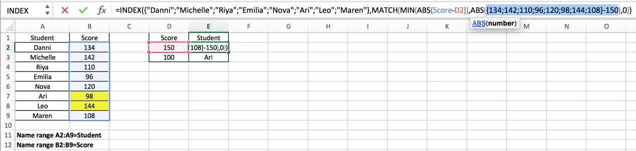
Calculate (Score-D2) in Excel formula bar and get below array:
{-16;-8;-40;-54;-30;-52;-6;-42}
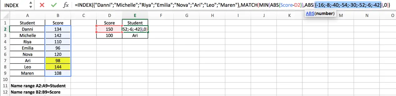
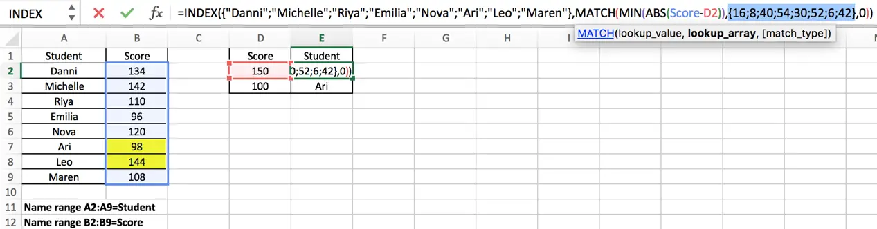
Use Excel ABS function to convert all negative numbers to positive numbers.
{16;8;40;54;30;52;6;42} – This array is the lookup array for MATCH function
For MIN(ABS(Score-D2)), the result of ABS function (numbers in the array above) is also delivered to MIN function:
=MIN({16;8;40;54;30;52;6;42})
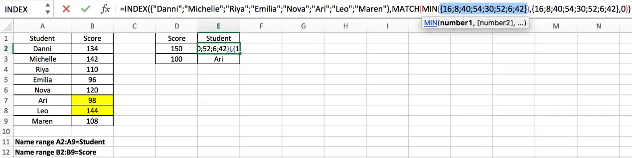
The Excel MIN function will extract the smallest value in the array.
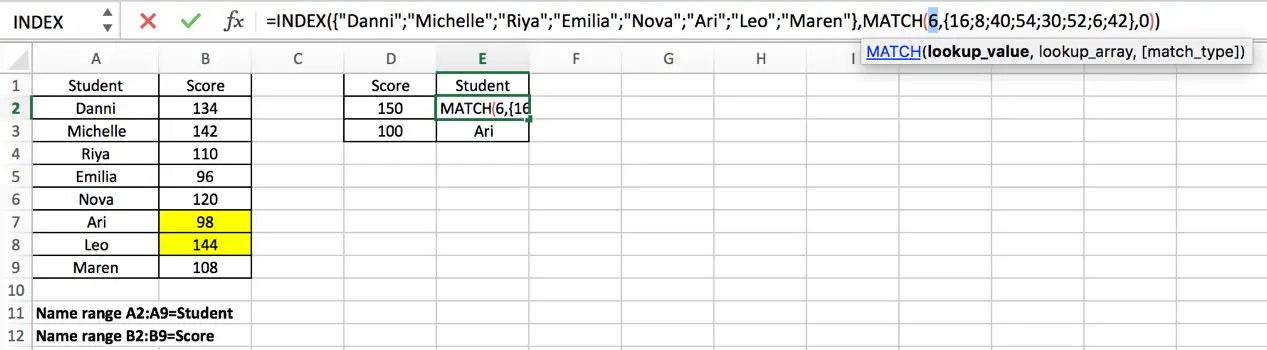
Now, for MATCH function, the lookup value and lookup array are obtained after calculating ABS and MIN expressions.
=MATCH(6,{16;8;40;54;30;52;6;42},0)
As mentioned above, Excel MATCH function returns the position of a certain value, so in this case, MATCH function returns the row number of value “6” in array {16;8;40;54;30;52;6;42}. Obviously, relative to this array, 6 is in row 7.
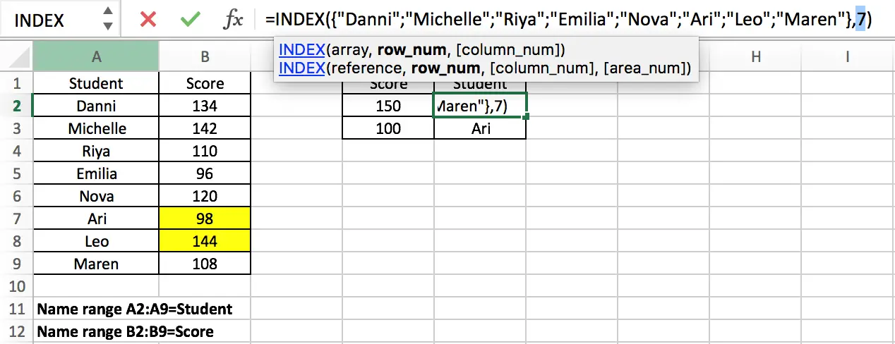
Now we come to the outermost INDEX function:=INDEX({“Danni”;”Michelle”;”Riya”;”Emilia”;”Nova”;”Ari”;”Leo”;”Maren”},7)
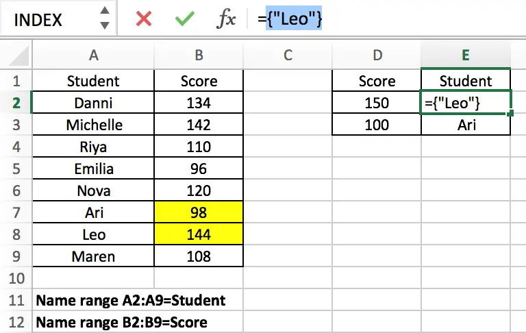
In this formula, MATCH function delivered row number 7 to INDEX function, INDEX function returns a value in an array based on a provided row number. In this array which consists of student names, the seventh name is “Leo”, so this is the final result for this formula. After entering “Ctrl+Shift+Enter”, “Leo” is displayed in cell E2.
Copied down the formula to E2, we can obtain “Ari” in the same way.
This article not only introduces the joint application of INDEX and MATCH, but also the use of MIN and ABS functions, including how to apply the combination of MIN and ABS functions to find the minimum difference between values. Readers can design their own formulas according to the actual situation.
Related Functions
- Excel INDEX function
The Excel INDEX function returns a value from a table based on the index (row number and column number)The INDEX function is a build-in function in Microsoft Excel and it is categorized as a Lookup and Reference Function.The syntax of the INDEX function is as below:= INDEX (array, row_num,[column_num])… - Excel MATCH function
The Excel MATCH function search a value in an array and returns the position of that item.The MATCH function is a build-in function in Microsoft Excel and it is categorized as a Lookup and Reference Function.The syntax of the MATCH function is as below:= MATCH (lookup_value, lookup_array, [match_type])…. - Excel MIN function
The Excel MIN function returns the smallest numeric value from the numbers that you provided. Or returns the smallest value in the array.The MIN function is a build-in function in Microsoft Excel and it is categorized as a Statistical Function.The syntax of the MIN function is as below:= MIN(num1,[num2,…numn])…. - Excel ABS Function
The Excel ABS function returns the absolute value of a number.The ABS function is a build-in function in Microsoft Excel and it is categorized as a Math and Trigonometry Function.The syntax of the ABS function is as below:=ABS (number)…