Find and retrieve is a common basic operation in Google Sheets for tables. In out daily work, we may encounter this situation that some data was lost after several operations on a table in Google Sheets. In fact, we can find the missing values by retrieving the original data and comparing it with the existing data.
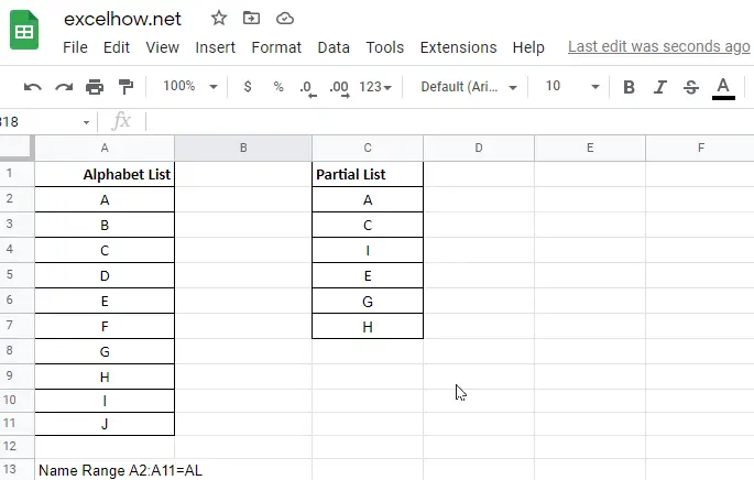
In this article, we will show you how to find and retrieve the missing values in Google Sheets. Look at the following example, compared to the initial column “Alphabet“, the “Partial List” only lists some letters, some are missing. What we need to do is to find the missing values and fill them in the “partial list” after the letter “H”.
Initial columns:
Expect result:
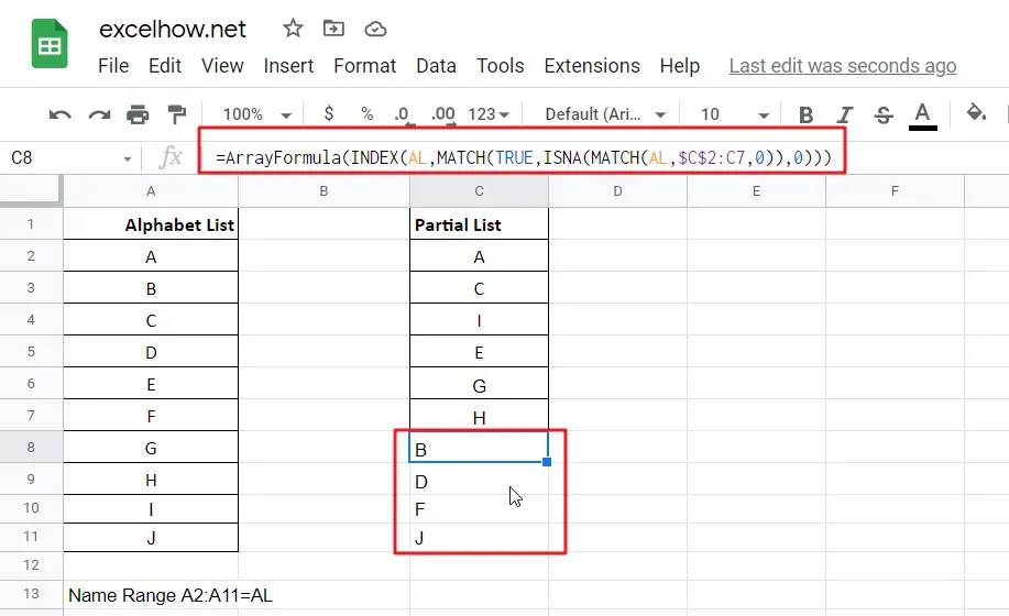
Table of Contents
General Formula in Google Sheets
The general formula for this case is as below:
=INDEX(CompleteList,MATCH(TRUE,ISNA(MATCH(CompleteList,PartialList,0)),0))
In the general Google Sheets formula, you can replace CompleteList and PartialList with your own table. This is an array formula, we need to enter “control + shift + enter” after entering the formula.
In the above example, the formula is:
=INDEX(AL,MATCH(TRUE,ISNA(MATCH(AL,$C$2:C7,0)),0))
The complete list is “Alphabet list” (A2:A11, named “AL”); Partial list is “Partial List” (C2:C7), this column is C2:C11 actually, but some values are missing, we need to refer to the complete list to fill in the missing values in cells C8:C11. Build above formula in C8, then copy down the formula, the missing values are pasted.
EXPLANATION
The general formula nests multiple formulas, and we need to explain each formula from inside to outside. The core is the internal MATCH function which helps us locate the missing values.
INDEX and MATCH
First let’s get to know the MATCH function.
MATCH is a Google Sheets function for locating the position of a query value in a row, column, or table. It supports approximate and exact matches, as well as partial matches with wildcards. Typically, MATCH is used in combination with the INDEX function to retrieve a value at a matching position.
The Syntax of the MATCH function is as below:
=MATCH (lookup_value, lookup_array, [match_type]) (match type 0=exact match)
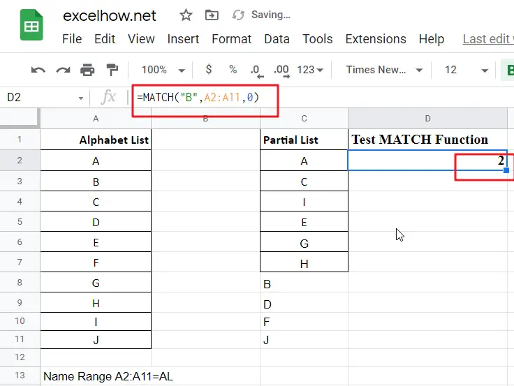
See the example below where MATCH returns the position of the letter “B” in the column.
=MATCH("B",A2:A11,0)
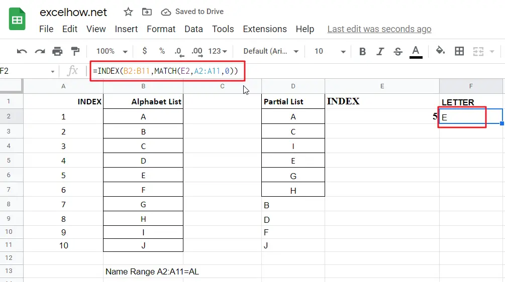
INDEX and MATCH Combination:
=INDEX(B2:B11,MATCH(E2,A2:A11,0))
In this example, we entered the formula in Cell C8:
=INDEX(AL,MATCH(TRUE,ISNA(MATCH(AL,$C$2:C7,0)),0))
Note: you need to entered “Shift+Control+Enter”, and formula returns missing letter B. You can find out letter B is the first missing letter among all missing letters in the list. As why B is returned in this cell, you can see our explanation in the following steps.
For expression MATCH(AL,$C$2:C7,0), refer to MATCH function syntax =MATCH (lookup_value, lookup_array, [match_type]), the lookup value is “AL” (A2:A11), the lookup array is $C$2:C7, as this formula will be copied down to cell C9 (until C11), so the lookup array is an extended range, the starting cell is a C2, so we add $ before row and column indexes; the ending cell is the cell “above it”, this allows the missing value returned from the formula (in cell C8 for example) is included in the next calculation (in cell C9), so we don’t need to add $ to lock the ending cell.
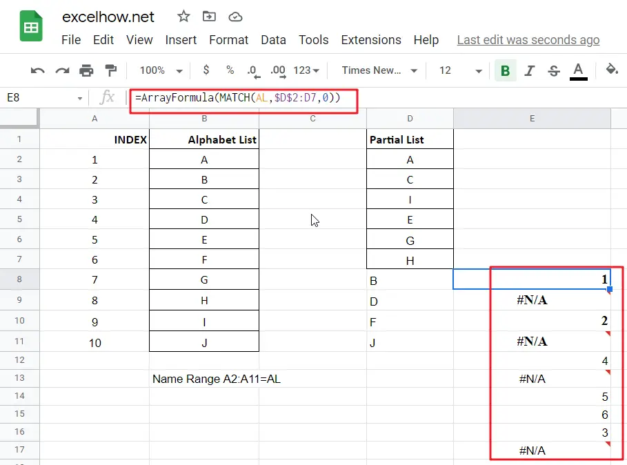
=ArrayFormula(MATCH(AL,$D$2:D7,0))
MATCH function will iterate through all the values in column “Alphabet List” and compares them against the column “Partial List”. It returns an array that contains numbers and #N/A errors.
In this example the result is:
{1;#N/A;2;#N/A;4;#N/A;5;6;3;#N/A}.
This array is directly delivered to ISNA function.
=ArrayFormula(ISNA(MATCH(AL,$D$2:D7,0)))
The ISNA function is used to determine if a value is a #N/A error. if it is, it returns true, if not, it returns false. In this example, if it is true, it represents a missing value, and if it is false, it represents an existing value. Based on the returned array of MATCH function, we can get a new array that only contains TRUE and FALSE after running ISNA.
The result of ISNA function:
{FALSE;TRUE;FALSE;TRUE;FALSE;TRUE;FALSE;FALSE;FALSE;TRUE}
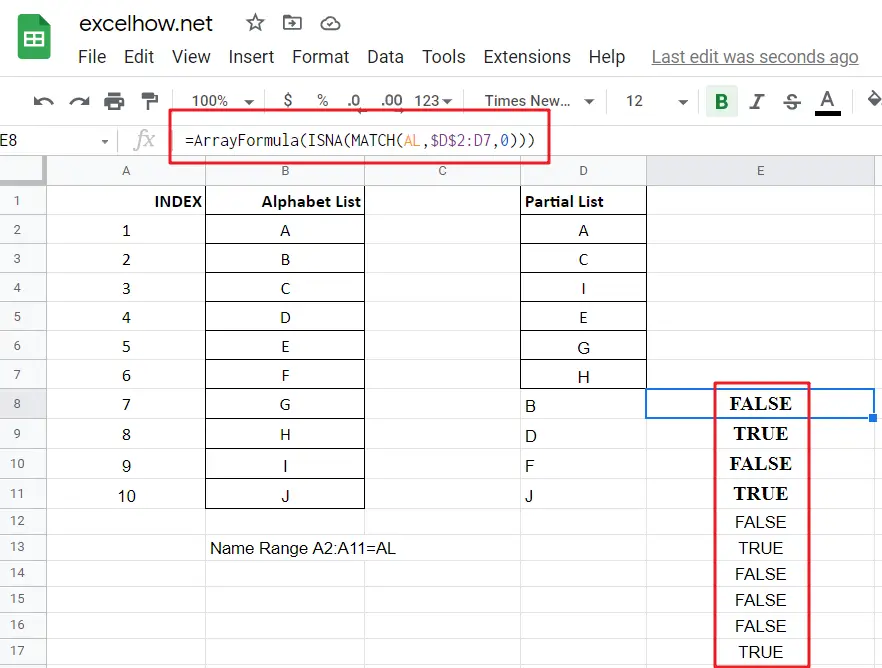
Refer to above screenshot, we can see that ISNA is the lookup array for the outer MATCH expression.
=ArrayFormula(MATCH(TRUE,ISNA(MATCH(AL,$D$2:D8,0)),0))
For this MATCH expression:
=MATCH(TRUE,{FALSE;TRUE;FALSE;TRUE;FALSE;TRUE;FALSE;FALSE;FALSE;TRUE},0)
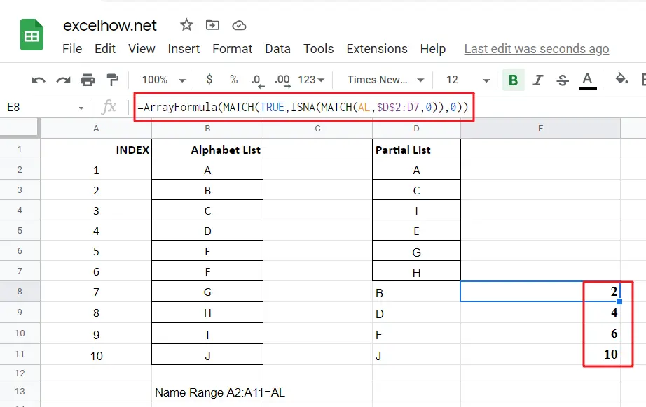
MATCH function will retrieve “TRUE” value from the lookup array and returns the first matching position of TRUE value. Obviously, the first TRUE value is listed in row 2.
=INDEX(AL,2)
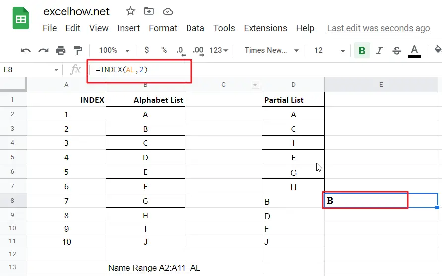
At last, INDEX function returns the letter in “row 2” in column AL. So letter B is returned in cell C8.
Copy down the formula to C9 (select cell C8, drag down the handler). Let’s see the result.
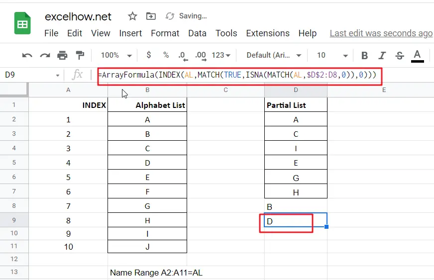
For the inner MATCH function, the lookup array is automatically extended to C8. Letter B is an existing letter in “Partial List”. Refer to above steps, the first missing value is D in this instance, so D is returned after running the formula.
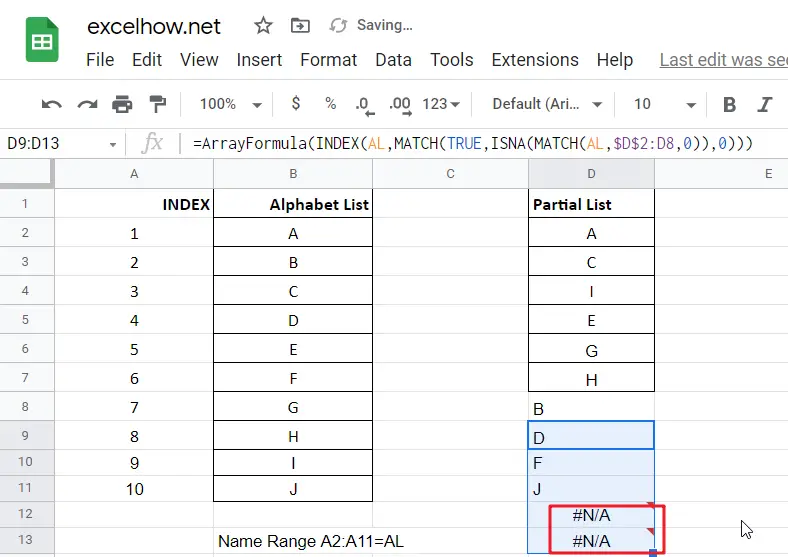
Notice: #N/A error will be returned after filling all missing values.
Related Functions
- Google Sheets INDEX function
The Google Sheets INDEX function returns a value from a table based on the index (row number and column number)The INDEX function is a build-in function in Google Sheets and it is categorized as a Lookup and Reference Function.The syntax of the INDEX function is as below:= INDEX (array, row_num,[column_num])… - Google Sheets MATCH function
The Google Sheets MATCH function search a value in an array and returns the position of that item.The MATCH function is a build-in function in Google Sheets and it is categorized as a Lookup and Reference Function.The syntax of the MATCH function is as below:= MATCH (lookup_value, lookup_array, [match_type])….