This post will guide you how to use Google Sheets INDEX function with syntax and examples.

Description

---

The Google Sheets INDEX function returns a value from a table based on the index (row number and column number). You can use INDEX function to extract entire rows or entire columns. This function is used to combine with the MATCH function to lookup value in a range or array.

The INDEX function can be used to extract the value at a given location in a range in google sheets. The purpose of this function is to get a value in a table based on a location, and the returned value is the value at a given location.

The INDEX function is a build-in function in Google Sheets and it is categorized as a Lookup function.

Syntax

---

There are two ways to use the INDEX function in excel:

If you want to get the value of a specified cell or array of cell, you can refer to Array form.

If you want to get a reference to specified cells, you can refer to Reference form.

The syntax of the INDEX function is as below:

= INDEX (array, row_num,[column_num])      #Array form

=INDEX(reference, row_num,[column_num],[area_num)     #Reference form

The array form is used in most cases, and if the first argument of the INDEX function is an array constant, you need to use the array form. If you want to perform a three-way lookup in a range, you can use the reference form.

Where the INDEX function arguments are:

• array -This is a required argument. A range of cells or data array. If array contains only one row or column, the corresponding row_num or Column_num argument is optional.
• Row_num – The row number in data array. If Row_num is omitted, column_num is required.
• Column_num – The column position in data array. If Column_num is omitted, row_num is required.
• Area_num – it is set as a number. If the first argument point to more cell ranges, if area_num is set to 1, then the first area will be selected.

Note:

• If you set the row_num and column_num at the same time, the INDEX function will return the value in the cell at the intersection of row number and column number.
• If you set the value of row_num or column_num to 0, the INDEX function will return the array of values for the entire row or column in the array data.
• Row_num and Column_num must point to a cell within array data, if not, the index function returns #REF!

Google Sheets INDEX Function Examples

---

The below examples will show you how to use google sheets INDEX function to return a value from a table based on the intersection of row number and column number.

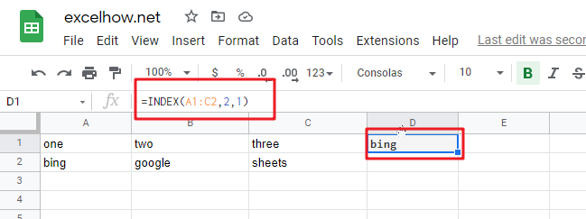
#1 To get the value at the intersection of the second row and second column in the table array: A1:C2, just using the following INDEX formula:

=INDEX(A1:C2,2,1)