This post will guide you how to use Google Sheets MATCH function with syntax and examples.

Description

---

The Google Sheets MATCH function search a value in an array and returns the position of that item.

The MATCH function can be used to get the position of an item in the given range or array in google sheets. Its returned value is a number that representing a position in a range.

The MATCH function is a build-in function in Google Sheets and it is categorized as a LOOKUP function.

Syntax

---

The syntax of the MATCH function is as below:

= MATCH(lookup_value, lookup_array, [match_type])

Where the MATCH function arguments are:

• Lookup_value -This is a required argument. The value that you want to search.
• Lookup_array – This is a required argument. The data array that is to be searched.
• Match_type – This is an optional argument. This value can be set as: 1, 0, -1. The default value is 1.

 Note:  

• 1 – the MATCH function will search the largest value that is less than or equal to Lookup_value
• 0 – The MATCH function will search the first value that is exactly equal to Lookup_value
• -1 – The Match function will search the smallest value that is greater than or equal to Lookup_value.
• MATCH function returns the position in an array or range of a matched value rather than the value itself. If you wish to return the value itself, and you need to use the INDEX function in combination with the MATCH function.

Google Sheets MATCH Function Examples

---

The below examples will show you how to use google sheets MATCH Function to get the position of an item in a range.

#1 =MATCH(35,A1:A4,1)

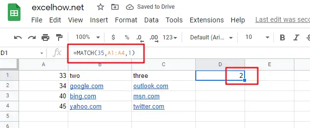
This MATCH Formula will search the value “35” and find the largest value that is less than or equal to “35”, it will return “2”, As the value “34” is the only largest value that is less than to “35”. It will return the position of value “34” in range “A1:A4”.

#2 =MATCH(35,A1:A4,0)

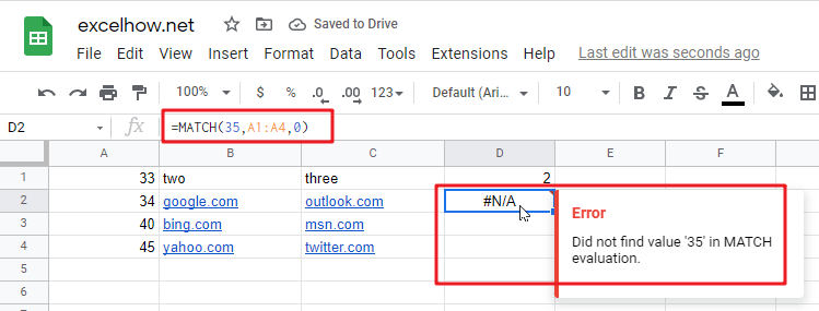
This Formula will return the “#N/A” value, As the matched type is set to “0”, it means that the function will find the first value that is exactly equal to “35”, but it is not able to find the value “35” in “A1:A4” range.

#3 =MATCH(35,A1:A4,-1)

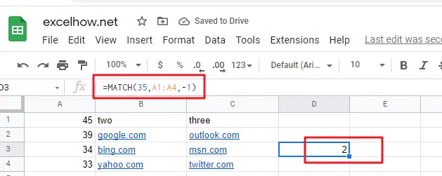
This Formula will return “2”, if the Match type is set to “-1”, the Match function will find the smallest value that is greater than or equal to “35”in range “A1:A4”, then return its position.