If you have a few values/items in the excel sheet and you are thinking that with the aid of the “VlOOKUP” function you can look for a specific value, extract it and then put the matching item into the separate column in Ms Excel easily, then congratulations, you are thinking right, but here a problem arises that there isn’t any doubt that by this way you can extract one or two matches into the separate column easily but with the aid of this way you cannot extract multiple matches into separate columns and if you would do that by this way then there are 90% chances that you would 100% get tired of it and can’t complete your task at the right time.
But don’t be worry about it because after carefully reading this article extracting multiple matches into the separate columns would become a piece of cake for you.
So let’s dive into the article to take you out of this fix.
Table of Contents
General Formula:
For extracting multiple matches(items) into seprate columns you can use the Array Formula which is based upon INDEX and SMALL, which is stated as follows:
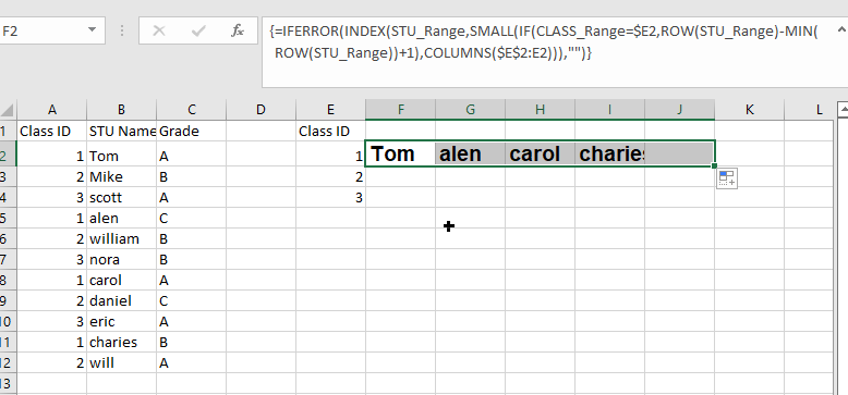
=IFERROR(INDEX(STU_Range,SMALL(IF(CLASS_Range=$E2, ROW(STU_Range) -MIN (ROW(STU_Range))+1),COLUMNS($E$2:E2))),"")
Syntax Explanations:
Before knowing about how to use this formula for getting the work done efficiently, we must understand each syntax which would make it easy for you that how each syntax contributes to extracting multiple matches into the separate columns:
IFERROR: This Function returns a custom result whenever a formula generates an error and returns the expected result when no error is detected.INDEX: In a range or array, this index function contributes to returning the value at a given position.SMALL: From the given range of data, this small Function returns the NthIF: In Excel, this IF Function contributes to returning two different values, one value for the TRUE result and another for the FALSE result.ROW: In Excel, this Row function contributes toreturning the row number as a reference.MIN: From the range of input values, this MIN function contributes to returning the smallest numeric value.Absolute Reference: The Absolute referenceis nothing but an actual fixed location in a worksheet.COLUMNS: From a given reference, this Column function contributes to counting the columns.Comma symbol (,): This symbol acts as a separator that contributes to separating a list of values.Minus Operator (-): This minus symbol contributes to subtracting any two values.Parenthesis (): The primary purpose of this parenthesis symbol is to group the various elements.Name– It represents the input ranges in your worksheet.Plus operator (+): This plus symbol adds the values.
Let’s See How This Formula Works:
To use this array formula for getting the work done, you must enter this formula with Control + Shift + Enter. As soon as you would enter this formula into the first cell, you need to drag it down and across to fill in the other cells.
As you can see in the above screenshot, this formula uses two names ranging: “ CLASS_Range ” and “ STU_Range,” where “ STU_Range ” refers to B2:B12 and on the other hand “ CLASS_Range ” refers to A2:A12.
You would definitely wonder that how this formula works to extract multiple matches into columns? So here is the answer. In this formula, we use the Small Function and INDEX function, which work together.
As the SMALL Function (dynamically constructed by IF) is used to obtain row number corresponding to an “nth match,” so after getting the row number from SMALL Function, this would then pass it into the INDEX function, which returns the value at that row, this is also the main motive of this formula.
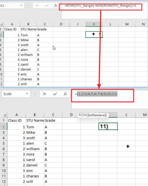
The snippet “IF(CLASS_Range=$E2, ROW(STU_Range) -MIN (ROW(STU_Range))+1” tests the named range “ STU_Range ” for the value in E2. If the value is found, then from an array of relative row numbers, it would return a row number, which is created with:
=ROW(STU_Range) -MIN (ROW(STU_Range))+1
The output of this formula is :
{1;2;3;4;5;6;7;8;9;10;11}
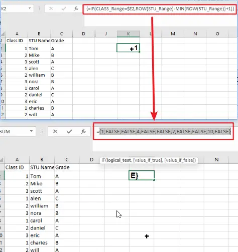
Now the final result is an array that would contain the numbers where there is a match, and FALSE where there is not any match found:
{1;FALSE;FALSE;4;FALSE;FALSE;7;FALSE;FALSE;10;FALSE}
Then this array goes into the SMALL Function. By expanding range(Given Below), The k value for SMALL (nth) returns:
COLUMNS($E$2:E2)
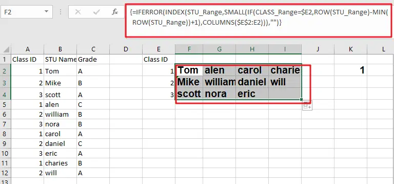
The SMALL function returns each matching row number, which is then supplied as the row_num to the INDEX function as the array with the range named “ STU_Range.”
Notes:
Now, this question would pop up in your mind that how would it handle the errors? Then whenever the COLUMN would return a value for k that does not exist, the #NUM error would be thrown by the SMALL Function at the next moment. This usually occurs when all the matches have occurred. To tackle the errors, the formula is wrapped up in the Function named “IFERROR,” which would receive the errors and then return an empty string (” “).
Related Functions
- Excel INDEX function
The Excel INDEX function returns a value from a table based on the index (row number and column number)The INDEX function is a build-in function in Microsoft Excel and it is categorized as a Lookup and Reference Function.The syntax of the INDEX function is as below:= INDEX (array, row_num,[column_num])… - Excel MATCH function
The Excel MATCH function search a value in an array and returns the position of that item.The MATCH function is a build-in function in Microsoft Excel and it is categorized as a Lookup and Reference Function.The syntax of the MATCH function is as below:= MATCH (lookup_value, lookup_array, [match_type])…. - Excel IF function
The Excel IF function perform a logical test to return one value if the condition is TRUE and return another value if the condition is FALSE. The IF function is a build-in function in Microsoft Excel and it is categorized as a Logical Function.The syntax of the IF function is as below:= IF (condition, [true_value], [false_value])…. - Excel ROW function
The Excel ROW function returns the row number of a cell reference.The ROW function is a build-in function in Microsoft Excel and it is categorized as a Lookup and Reference Function.The syntax of the ROW function is as below:= ROW ([reference])…. - Excel SMALL function
The Excel SMALL function returns the smallest numeric value from the numbers that you provided. Or returns the smallest value in the array.The syntax of the SMALL function is as below:=SMALL(array,nth) … - Excel MIN function
The Excel MIN function returns the smallest numeric value from the numbers that you provided. Or returns the smallest value in the array.The MIN function is a build-in function in Microsoft Excel and it is categorized as a Statistical Function.The syntax of the MIN function is as below:= MIN(num1,[num2,…numn])…. - Excel IFERROR function
The Excel IFERROR function returns an alternate value you specify if a formula results in an error, or returns the result of the formula.The syntax of the IFERROR function is as below:= IFERROR (value, value_if_error)…. - Excel COLUMN function
The Excel COLUMN function returns the first column number of the given cell reference.The syntax of the COLUMN function is as below:=COLUMN ([reference])….