Suppose that you are working with two lists containing few values, and you want to extract the matching values from those two lists into another separate list. You might prefer to manually extract the matching values from the two lists, which is ok for the few values, but it would be a big deal to extract the matching values from the two lists having multiple cells, and doing it manually would be a foolish attempt because there are 90% chances that you would 100% get tired of it and would never complete your work on time.
But don’t be worry about it because after carefully reading this article, extracting the matching values from the two lists into another separate list would become a piece of cake for you.
So let’s dive into the article to take you out of this fix.
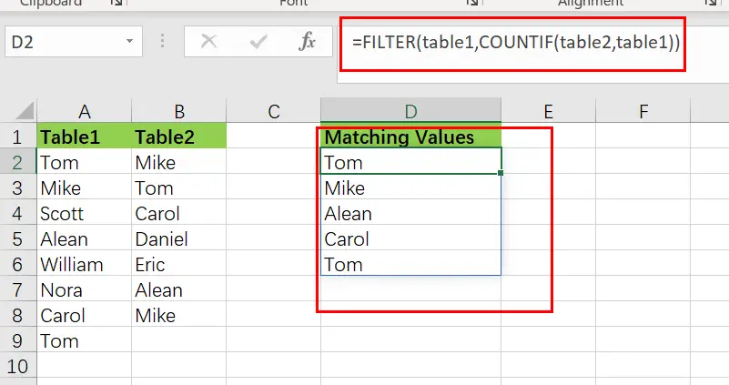
Table of Contents
General Formula
The Following Formula would help you compare and extract the matching values from the two lists into another separate list.
=FILTER(table1,COUNTIF(table2,table1))
This Formula is based on the FILTER and COUNTIF functions, where the table1(A2:A9) and table2 (B2:B8) are the named ranges, the list in the range (D2:D6) is the list containing the matching values by comparing both table1 and table2.
Syntax Explanations
Before going into the explanation of the Formula for getting the work done efficiently, we must understand each syntax which would make it easy for you that how each syntax contributes to executing the matching values from the two lists into another separate list:
Filter: This function contributes to narrowing down or filtering out a range of data on the user-defined criteria.COUNTIF: It is a statistical function that counts the number of cells to meet specific criteria.List: In this Formula, the list represents the two lists present in the excel worksheet to execute the common values.Comma symbol (,): In Excel, this comma symbol acts as a separator that helps to separate a list of values.Parenthesis (): The core purpose of this Parenthesis symbol is to group the elements and separate them from the rest of the elements.
Let’s See How This Formula Works
The FILTER function is used in this Formula to extract data based on a logical test created using the COUNTIF function:
=FILTER(table1,COUNTIF(table2,table1))
The COUNTIF function is being used to generate the actual filter.
=COUNTIF(table2,table1))
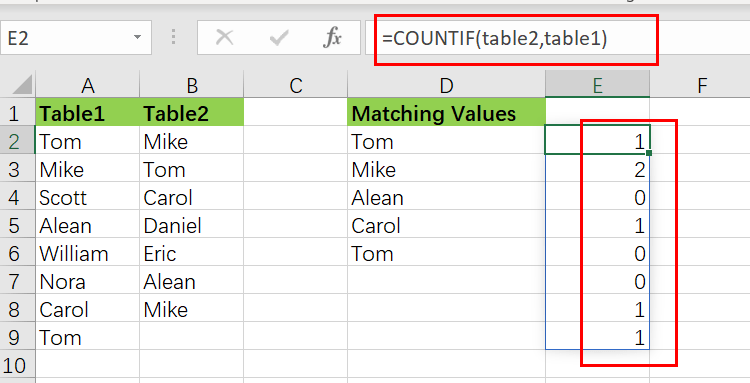
It’s worth noticing that we’re using table2 as the range argument and table1 as the criterion argument. In other words, we’re asking COUNTIF to count all values in table1 that occur in table2. We obtain an array with several results since we provide COUNTIF various values for criteria:
{1;2;0;1;0;0;0;1}
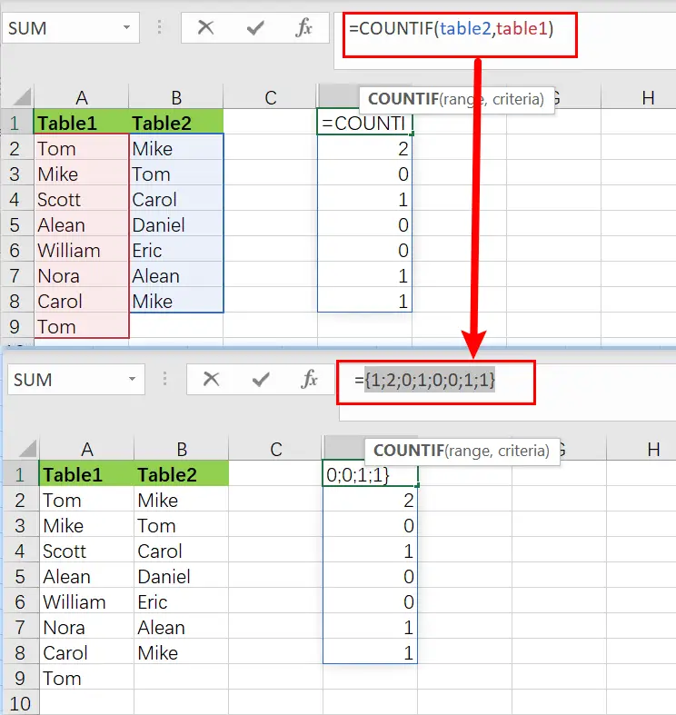
Note that the array has 8 counts for each element in the table1. A zero value denotes a value in a table1 that is not present in the table2. Any other positive number denotes a value in table1 that is also present in table2. As the include parameter, this array is passed straight to the FILTER function:
=FILTER(table1,{1;1;0;1;0;1;0;0;1;0;1;1})
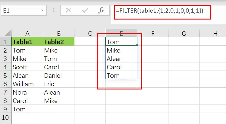
The array is used as a filter by the filter function. Any item in the table1 connected with a zero would be eliminated, but any value related to a positive number would retain.
Extract Non-matching Values
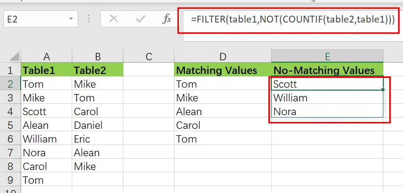
If you want to remove the non-matching values from table1, values in table1 that do not present in table2, we would need to modify the above formula, which is stated as follows:
=FILTER(table1,NOT(COUNTIF(table2,table1)))
The NOT function reverses the COUNTIF result, and every non-zero integer returns FALSE, and any zero value returns TRUE. The output is a list of all the values in the table1 that aren’t on the table2.
Method two: Extract Matching Values Using INDEX
You can also create a newly formula to extract matching values without the FILTER function, but the Formula would become more complicated. And the formula based on the INDEX function. Like below:
=IFERROR(INDEX(table1,SMALL(IF(COUNTIF(table2,table1),ROW(table1)-ROW(INDEX(table1,1,1))+1),ROWS($D$2:D2))),"")
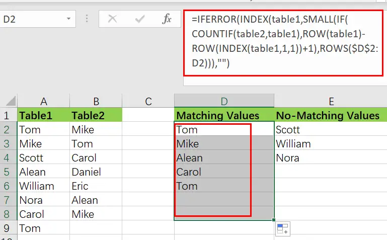
Except in Excel 365, this array formula must be typed using control + shift + enter.
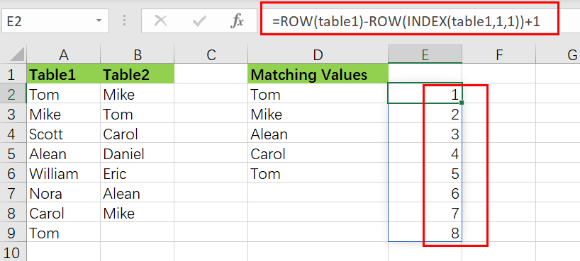
The INDEX function, which takes table1 as an array parameter, lies at the heart of this Formula. The majority of the remaining Formula determines the row number for matching values. This expression creates a list of relative row numbers as follows:
=ROW(table1)-ROW(INDEX(table1,1,1)) +1
which yields a 12-number array reflecting the rows in table1:
{1;2;3;4;5;6;7;8;}
These are filtered using the IF function and the same methodology used above in the FILTER Function, but this time using the COUNTIF function:
=COUNTIF(table2,table1) / identify values that match
=IF(COUNTIF(table2,table1),ROW(table1)-ROW(INDEX(table1,1,1))+1)
The resultant array is as follows:
{1;2;FALSE;4;FALSE; FALSE;7;8; }
As the Formula is copied along the column, this array is sent immediately to the SMALL function.
The IFERROR function is designed to catch mistakes when a formula is copied down, and the matching values run out.
Related Functions
- Excel COUNTIF function
The Excel COUNTIF function will count the number of cells in a range that meet a given criteria. This function can be used to count the different kinds of cells with number, date, text values, blank, non-blanks, or containing specific characters.etc.= COUNTIF (range, criteria)… - Excel Filter function
The FILTER function extracts matched records from a collection of data using one or more logical checks. The include argument specifies logical tests, which might encompass a wide variety of formula conditions.==FILTER(array,include,[if empty])… - Excel INDEX function
The Excel INDEX function returns a value from a table based on the index (row number and column number)The INDEX function is a build-in function in Microsoft Excel and it is categorized as a Lookup and Reference Function.The syntax of the INDEX function is as below:= INDEX (array, row_num,[column_num])… - Excel IF function
The Excel IF function perform a logical test to return one value if the condition is TRUE and return another value if the condition is FALSE. The IF function is a build-in function in Microsoft Excel and it is categorized as a Logical Function.The syntax of the IF function is as below:= IF (condition, [true_value], [false_value])…. - Excel ROW function
The Excel ROW function returns the row number of a cell reference.The ROW function is a build-in function in Microsoft Excel and it is categorized as a Lookup and Reference Function.The syntax of the ROW function is as below:= ROW ([reference])…. - Excel SMALL function
The Excel SMALL function returns the smallest numeric value from the numbers that you provided. Or returns the smallest value in the array.The syntax of the SMALL function is as below:=SMALL(array,nth) … - Excel IFERROR function
The Excel IFERROR function returns an alternate value you specify if a formula results in an error, or returns the result of the formula.The syntax of the IFERROR function is as below:= IFERROR (value, value_if_error)…. - Excel NOT function
The Excel NOT function returns the opposite of a given logical or Boolean value. For example, if you supplied with the value TRUE, the NOT function will return FALSE; If you supplied with the value FALSE, and the NOT function will TRUE. The syntax of the NOT function is as below:=NOT(logical)…