Today, we will show you how to use SUMPRODUCT and EXACT to perform a case sensitive exact match. In this article, we provide a simple example to calculate bonus for employees whose names are case-sensitive. If you meet similar scenarios in your daily work, you can directly use this formula to deal with your problem.
EXAMPLE
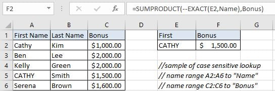
In this example, first name “Cathy” and “CATHY” are duplicate but they have different last name. To calculate bonus for “CATHY” correctly, we need to ignore “Cathy” from the list and find out “CATHY” properly, then retrieve bonus “$1,500.00” from cell C5 properly. To solve this problem, we can create a formula that can perform case-sensitive lookup and retrieves data from a particular position based on the lookup value.
Before creating the formula, to make cell reference and range reference used in the formula are easy to understand, we named range (A2:A6) to “Name”, (C2:C6) to “Bonus”. In this example, we will apply SUMPRODUCT function together with EXACT to perform an exact match.
ANALYSIS
The formula can perform below operations:
1. It can scan values from “First Name” column and find out lookup value “CATHY” properly.
2. As we have two “Cathy”, we need to ignore the first “Cathy”. Because for the first one, except the first letter, other letters are entered in lowercase. But for our input value “CATHY”, all five letters are entered in UPPERCASE. They are different if case sensitive.
3. After confirming the position of “CATHY”, it can retrieve data from “Bonus” column in the same row of “CATHY”.
4. It returns proper bonus get in step#3 after performing the formula.
Actually, there are some powerful functions and function combinations that can perform lookup effectively and powerfully, for example VLOOKUP function or INDEX/MATCH function combination. However, no matter VLOOKUP function or INDEX/MATCH functions, they are not case-sensitive functions. They will return the first match result ignoring case. So, we need the help from other functions that are case-sensitive and can perform case-sensitive comparison properly. In Excel, EXACT is frequently used for case-sensitive comparison, so, in this example, we will create a formula with EXACT function. At the core, this is a SUMPRODUCT formula, EXACT is applied inside SUMPRODUCT function to perform case-sensitive comparison.
The formula: SUMPRODUCT(–EXACT(E2,Name),Bonus)
FORMULA
Input formula =SUMPRODUCT(–EXACT(E2,Name),Bonus) into F2. As this is an array formula, so we must press Control+Shift+ENTER to return result. Verify that “$1,500.00” is displayed properly.
FUNCTION INTRODUCTION
a. SUMPRODUCT function can be seen as SUM+PRODUCT. It returns the sum of products of corresponding ranges or arrays.
Syntax:
=SUMPRODUCT(array1,array2,array3, ...)
b. EXACT function is case-sensitive, it can detect whether two strings are exactly the same. If yes, it returns TRUE, else it returns FALSE.
Syntax:
=EXACT(text1, text2)
EXPLANATION
=SUMPRODUCT(--EXACT(E2,Name),Bonus)
a. EXACT(E2,Name) performs a case-sensitive comparison between value in E2 (“CATHY”) and values in “Name”({“Cathy”;”Ben”;”Kelly”;”CATHY”;”Serena”}). It returns “TRUE” if the two strings are exactly the same. So, after comparison, we get below an array of “TRUE” and “FALSE”:
{FALSE;FALSE;FALSE;TRUE;FALSE}
Select EXACT(E2,Name) in the formula bar and press F9, you can see the result returned by EXACT function:
![]()
b. We add double negative to coerce “TRUE” into number “1” and FALSE into number “0”. Then we get below array consists of numbers “1” and “0”:
{0;0;0;1;0}
Select –{FALSE;FALSE;FALSE;TRUE;FALSE} and press F9:
![]()
c. {0;0;0;1;0} is delivered to SUMPRODUCT function as one array. In this array, “1” represents “CATHY”, its position in the array reflects the position of “CATHY” in range “Name”.
d. Expand values in “Bonus”:
{1000;2000;2000;1500;1600}
Select “Bonus” and press F9:
![]()
SUMPRODUCT multiplies the items in each array and get result {0;0;0;1500;0}; Then returns sum of product: 1500.
NOTICE
1. SUMPRODUCT only works when items are numeric values in each array. So, in this case, if values in named range “Bonus” are texts, SUMPRODUCT doesn’t work. If you want to retrieve text, you can apply VLOOKUP or INDEX/MATCH with EXACT function.
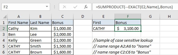
2. This formula doesn’t work properly if there are multiple matches. It will return the sum of all matches. For example, two “CATHY”.
Related Functions
- Excel INDEX function
The Excel INDEX function returns a value from a table based on the index (row number and column number)The INDEX function is a build-in function in Microsoft Excel and it is categorized as a Lookup and Reference Function.The syntax of the INDEX function is as below:= INDEX (array, row_num,[column_num])… - Excel MATCH function
The Excel MATCH function search a value in an array and returns the position of that item.The MATCH function is a build-in function in Microsoft Excel and it is categorized as a Lookup and Reference Function.The syntax of the MATCH function is as below:= MATCH (lookup_value, lookup_array, [match_type])…. - Excel EXACT function
The Excel EXACT function compares if two text strings are the same and returns TRUE if they are the same, Or, it will return FALSE.The syntax of the EXACT function is as below:= EXACT (text1,text2)… - Excel VLOOKUP function
The Excel VLOOKUP function lookup a value in the first column of the table and return the value in the same row based on index_num position.The syntax of the VLOOKUP function is as below:= VLOOKUP (lookup_value, table_array, column_index_num,[range_lookup])…. - Excel SUMPRODUCT function
The Excel SUMPRODUCT function multiplies corresponding components in the given one or more arrays or ranges, and returns the sum of those products.The syntax of the SUMPRODUCT function is as below:= SUMPRODUCT (array1,[array2],…)…