Suppose you got a task to calculate the win, loss, and tie totals; what would you do? If you are new to Ms Excel and don’t have enough experience with it, then you might do this task manually but let me add that doing this task manually would take a lot of time you will not be able to complete the task at a specific time and you will end up exhausted.

So for calculating a lot of win, loss, and tie totals in a matter of seconds, all you need to do is to read this article thoroughly

So without any further ado, let’s dive into it.

General Formula

Use the method below to compute win-loss tie totals.

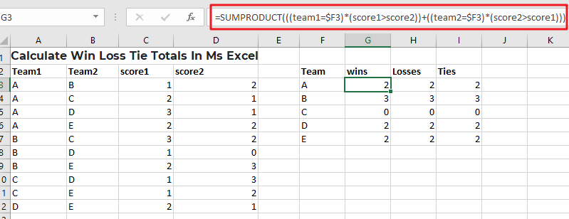
=SUMPRODUCT(((team1=$F3)*(score1>score2))+((team2=$F3)*(score2>score1)))

Syntax Explanation

• Parenthesis (): This symbol is used to organize the elements.
• Plus operator (+): This symbol aids in the addition of values.
• SUMPRODUCT: In Excel, this function multiplies the relevant arrays or ranges and returns the total of the products. More information on the SUMPRODUCT Function may be found here.

Summary 

A formula based on the SUMPRODUCT function may be used to determine a team’s win, loss, and tie totals using game data that contains a score for both sides. Type the following formula:

=SUMPRODUCT(((team1=$F3)*(score1>score2))+((team2=$F3)*(score2>score1)))

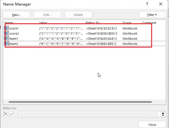
Based on the data presented, this formula gives total wins for the “A”  team and set the following are the named ranges: team1 (A3:A12), team2 (B3:B12), score1 (C3:C12), and score2 (D3:D12).

Let’s See How This Formula Works:

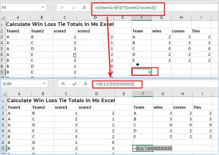
In this example, the purpose is to compute total wins, losses, and ties for each team mentioned in column F. The fact that a team can appear in either column A or B complicates matters significantly; therefore, we must account for this when computing wins and losses.

You may consider utilizing the COUNTIF or COUNTIFS function to solve this problem. However, these methods are limited to dealing with established ranges for criteria. Instead, the example formula uses the SUMPRODUCT function to sum the result of a Boolean logic-based array expression. When a team occurs in column A, we use the following equation within SUMPRODUCT on the left:

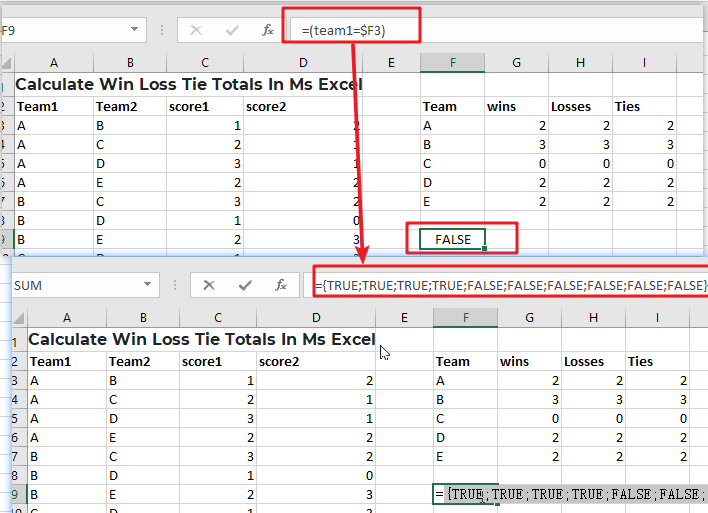
=((team1=$F3)*(score1>score2))

This expression comprises two expressions connected by multiplication (*) to construct AND logic.

=(team1=$F3) / It will verify that if the team is “A”

The equation on the right determines whether or not the score1 is larger than the score2:

=(score1>score2) / ensure that score1 is larger than the score2.

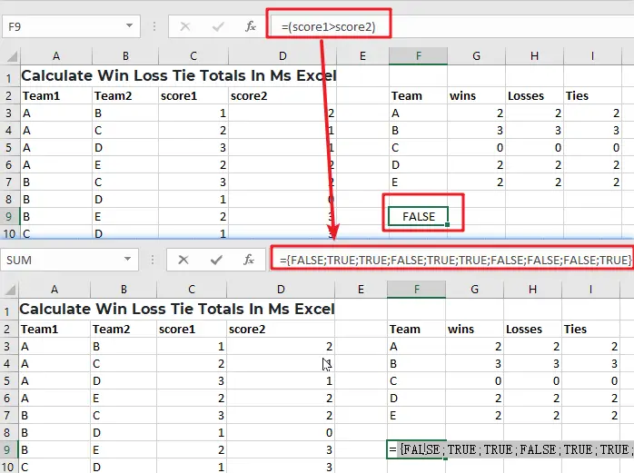
Because both expressions utilize multiple-valued ranges, they both yield arrays with numerous outcomes. When we rewrite the formula with the arrays returned.

Multiplication (*) is a math operation that, like AND in Boolean algebra, converts TRUE and FALSE values into 1s and 0s. When both of the related values are TRUE, the outcome is 1. In all other cases, the answer is 0. The end result is a single array that looks like the following:

We have identical reasoning on the right side that checks for Team A wins when A is Team 2:

=((team2=$F3)*(score2>score1)))

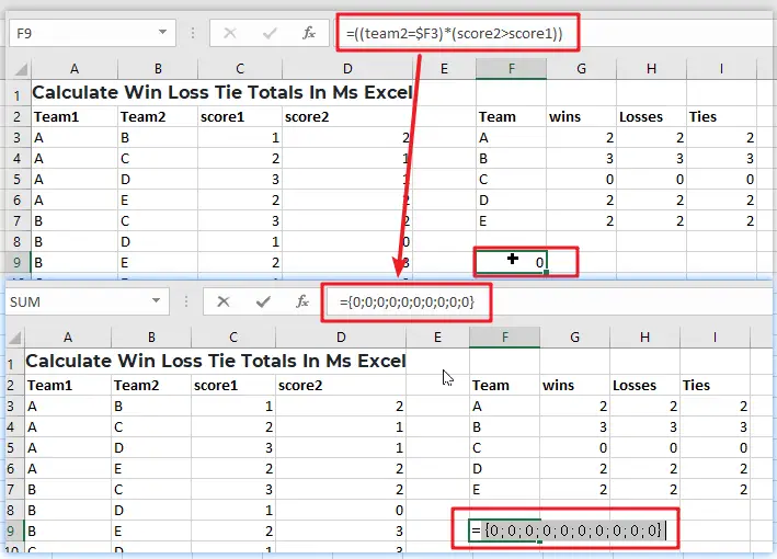
Because “A” does not appear as Team 2 in any game, all results are 0.

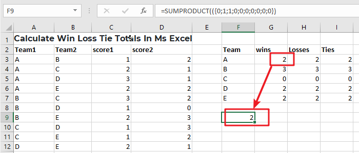
After evaluating both the left and right sides, we can rewrite the original formula as follows:

=SUMPRODUCT(({0;1;1;0;0;0;0;0;0;0})+({0;0;0;0;0;0;0;0;0;0}))

Notice that the arithmetic operator between the two arrays is addition (+), which corresponds to OR logic at this point. We do this because A wins as either Team 1 or Team 2. The result is a single array within SUMPRODUCT:

=SUMPRODUCT(({0;1;1;0;0;0;0;0;0;0})

 With only one array to process, SUMPRODUCT adds the array’s components and provides a single result, 2.

Related Functions

• Excel SUMPRODUCT function
  The Excel SUMPRODUCT function multiplies corresponding components in the given one or more arrays or ranges, and returns the sum of those products.The syntax of the SUMPRODUCT function is as below:= SUMPRODUCT (array1,[array2],…)…
• Excel COUNTIF function
  The Excel COUNTIF function will count the number of cells in a range that meet a given criteria. This function can be used to count the different kinds of cells with number, date, text values, blank, non-blanks, or containing specific characters.etc.= COUNTIF (range, criteria)…
• Excel COUNTIFS function
  The Excel COUNTIFS function returns the count of cells in a range that meet one or more criteria. The syntax of the COUNTIFS function is as below:= COUNTIFS(criteria_range1, criteria1, [criteria_range2, criteria2]…)…