Suppose you got a task to adjust the values that contain the ties; what would be your first attempt to break the ties of the given value? If you are wondering about doing this task manually, let me add that you will end up exhausted, and there is a probability that you will not complete this task on time. Moreover, besides consuming a lot of time and energy, it also seems to be a cumbersome task to break the ties in the values manually.
But don’t worry about it because you have just landed on the right article, where you will get concise information to break the ties in just a matter of seconds.
So without any further ado, let’s get started.
Table of Contents
General formulation
The formula for breaking ties in values using column and COUNTIF is as follows.
= (COUNTIF(range,A1)-1)*adjustment + A1
Explanation of Syntax
You must be aware of the syntax used in the above formula to use it to complete your task.
CountIF: In Excel, the COUNTIF function counts the number of cells that fulfill a specific condition or criteria. Learning how to utilize the COUNTIF Excel function is helpful because we frequently want to know how many objects in a huge collection are alike in a specific manner. The COUNTIF function is commonly used as a fast fix.
- The plus operator (+): This operator is used to add the values.
- Minus Operator (-): Use this symbol to subtract any two numbers.
- Multiplication (*): In this symbol, any two values or numbers will be multiplied.
- The comma symbol (,): This symbol is a separator that aids in the separation of a list of values.
- Parenthesis (): This symbol’s primary function is to group the elements.
Summary
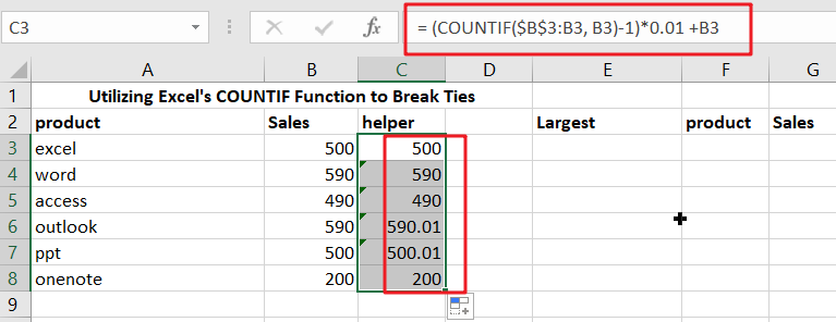
To break ties, use a helper column and the COUNTIF function to alter values so that they don’t have duplicates and don’t result in ties. The formula in D5 in the example is:
= (COUNTIF($B$3: B3, B3)-1)*0.01 +B3
When you employ SMALL, LARGE, or RANK functions to rank highest and lowest values, you may encounter ties because the data contains duplicates. In this situation, one method for breaking ties is to create a helper column with altered values, then rank those values instead of the originals.
The reasoning used to alter values in this example is random – the first duplicate value will “win,” but you may modify the formula to employ appropriate logic for your specific scenario and use case.
Explanation
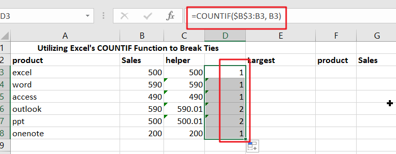
This formula relies on the COUNTIF function and an increasing range to count occurrences of values. COUNTIFS uses the expanding reference to deliver a running count of occurrences rather than a total count for each value:
=COUNTIF($B$3: B3, B3)
= (COUNTIF($B$3: B3, B3)-1)*0.01
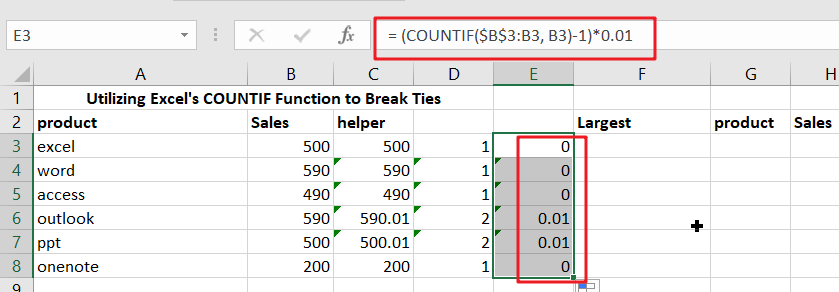
The result is then multiplied by 0.01 after being removed by 1 (which makes the count of all non-duplicate values zero). This is the “adjustment,” It is purposefully minimal to not significantly influence the original value.
“excel” and “ppt” both have the same sales of 500 in the scenario. Because excel is first in the list, the running count of 500 equals 1 and is canceled out by removing 1; thus, the estimate in the helper column remains unchanged:
However, the running count of 500 for ppt product is 2, therefore the estimate is adjusted:
=B7+0.01
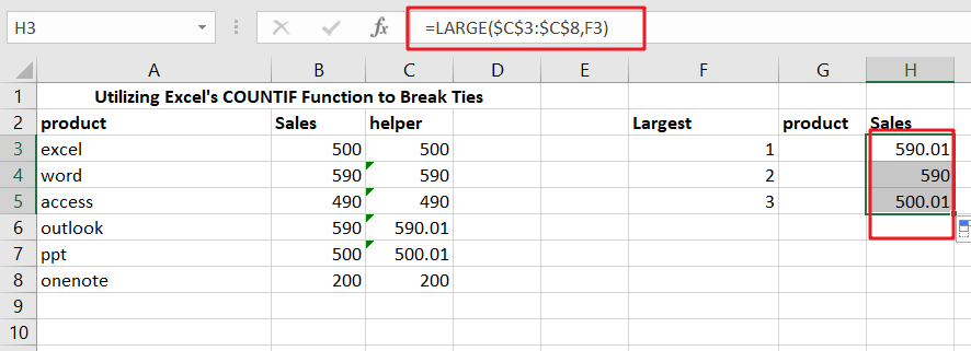
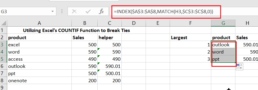
Finally, instead of the original values in columns G and H, the corrected values are utilized for ranking. The formula in H3.
=LARGE($C$3:$C$8,F3)
G3’s formula is as follows:
=INDEX($A$3:$A$8,MATCH(H3,$C$3:$C$8,0))
Column of temporary assistance
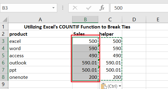
Suppose you don’t want to use a helper column in the final solution. In that case, you can use it temporarily to get calculated values, then use Paste Special to convert values into the original cell range.
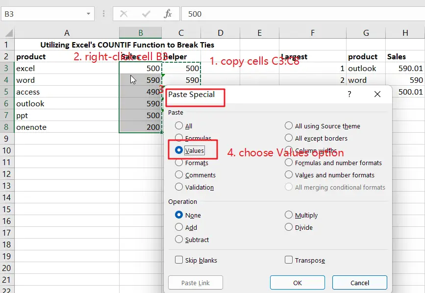
Then you can delete the helper column.
Related Functions
- Excel INDEX function
The Excel INDEX function returns a value from a table based on the index (row number and column number)The INDEX function is a build-in function in Microsoft Excel and it is categorized as a Lookup and Reference Function.The syntax of the INDEX function is as below:= INDEX (array, row_num,[column_num])… - Excel MATCH function
The Excel MATCH function search a value in an array and returns the position of that item.The MATCH function is a build-in function in Microsoft Excel and it is categorized as a Lookup and Reference Function.The syntax of the MATCH function is as below:= MATCH (lookup_value, lookup_array, [match_type])…. - Excel COUNTIF function
The Excel COUNTIF function will count the number of cells in a range that meet a given criteria. This function can be used to count the different kinds of cells with number, date, text values, blank, non-blanks, or containing specific characters.etc.= COUNTIF (range, criteria)… - Excel LARGE function
The Excel LARGE function returns the largest numeric value from the numbers that you provided. Or returns the largest value in the array. The syntax of the LARGE function is as below:= LARGE (array,nth)…