As an MS Excel user, you might have come across a task where you need to abbreviate different names or words, and there are also possibilities that you might have done this task manually by assuming that there isn’t any other way to do this task, but you assumed wrong because fortunately there is a way which would let you abbreviate names and words in a matter of seconds unlike doing it manually which consumes a lot of time and leaves you with no satisfying results.

So for exploring that way/method, let’s dive into the article.

General Formula:

The array formula to abbreviate different names and words in few seconds is mentionedas follows:

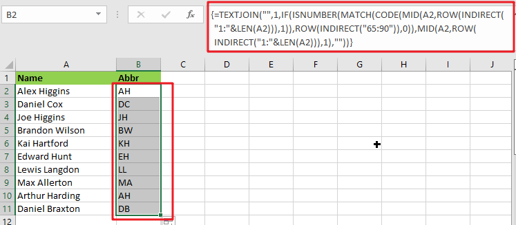
{=TEXTJOIN("",1,IF(ISNUMBER(MATCH(CODE(MID(A2,ROW(INDIRECT("1:"&LEN(A2))),1)),ROW(INDIRECT("65:90")),0)),MID(A2,ROW(INDIRECT("1:"&LEN(A2))),1),""))}

Syntax Explanation:

To understand the working of the above formula, we first need to know about each syntax and how they contribute to abbreviating names and words in seconds.

• TEXTJOIN: The TEXTJOIN function in Microsoft Excel allows you to join two or more strings together, with each value separated by a delimiter. The TEXTJOIN function is an Excel built-in function classified as a String/Text Function.
• IF: The IF function is one of Excel’s most used functions, allowing you to create logical comparisons between a number and what you anticipate.
• ISNUMBER: When a cell contains a number, the ISNUMBER function returns TRUE; otherwise, it returns FALSE. ISNUMBER can be used to verify that a cell contains a numeric value or that the output of another function is a number.
• MATCH: The MATCH is a function used to find a lookup value in a row, column, or table in MS Excel. MATCH allows for approximate and accurate matching and wildcards (*?) for partial matches.
• CODE: The CODE function in Excel returns a numeric code for a specified character.
• INDIRECT: The INDIRECT function returns a range reference. This function may generate a reference that will not change if a row or column is added to the worksheet.

Let’s See How This Formula Works:

To abbreviate capital letters text, use this array formula based on the TEXTJOIN function, new in Office 365 and Excel 2019. You may use this method to generate initials from names or acronyms. Because only capital letters can survive this algorithm, the original text must contain capitalized terms. If necessary, you can capitalize words using the PROPER function.

The formula in B2 in the case provided is:

=TEXTJOIN("",1,IF(ISNUMBER(MATCH(CODE(MID(A2,ROW(INDIRECT("1:"&LEN(A2))),1)),ROW(INDIRECT("65:90")),0)),MID(A2,ROW(INDIRECT("1:"&LEN(A2))),1),""))

The MID function is used to turn the string into an array of individual letters from the inside out:

=MID(A2,ROW(INDIRECT("1:"&LEN(A2))),1)

In this formula section, the operators MID, ROW, INDIRECT, and LEN transform a string into an array of letters.

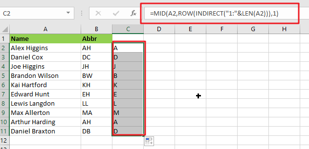
MID delivers an array of all characters in the text.

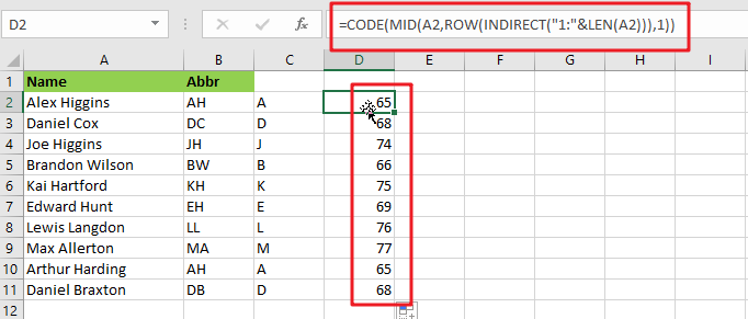
=CODE(MID(A2,ROW(INDIRECT("1:"&LEN(A2))),1))

This above array is sent to the CODE function, which returns an array of numeric ASCII codes, one for each letter.

=ROW(INDIRECT("65:90")

ROW and INDIRECT are used to generate another numeric array:

{65;66;67;68;69;70;71;72;73;74;75;76;77;78;79;80;81;82;83;84;85;86;87;88;89;90}

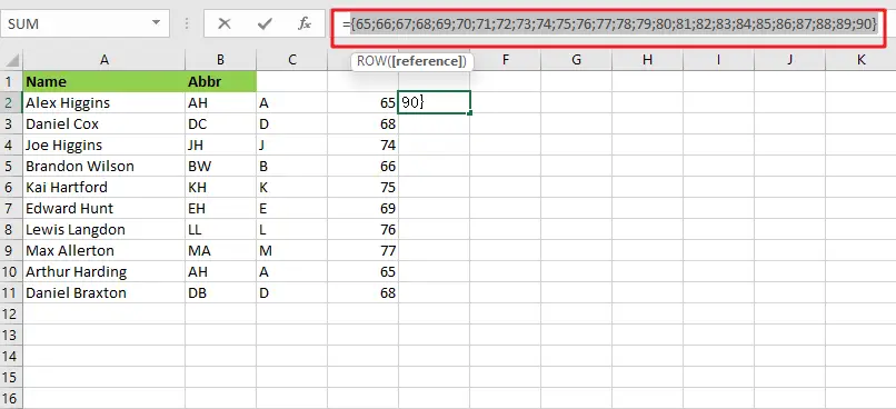
Note: The digits 65 to 90 correspond to the ASCII codes for all capital letters from A to Z. This array is used as the lookup array in the MATCH function, and the original array of ASCII codes is given as the lookup value.

{=MATCH(CODE(MID(A2,ROW(INDIRECT("1:"&LEN(A2))),1)),ROW(INDIRECT("65:90")),0)}

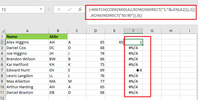
The MATCH function returns either a number or the #N/A error. Because numbers represent capital letters.

{=IF(ISNUMBER(MATCH(CODE(MID(A2,ROW(INDIRECT("1:"&LEN(A2))),1)),ROW(INDIRECT("65:90")),0)),MID(A2,ROW(INDIRECT("1:"&LEN(A2))),1),"")}

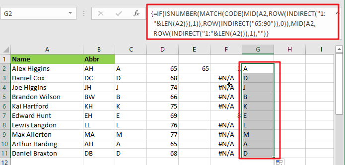
The ISNUMBER function is used with the IF function to filter results. Only characters with ASCII codes between 65 and 90 will be included in the final array, reconstructed using the TEXTJOIN method to produce the final abbreviation or acronym.

Abbreviate Names And Words In MS Excel 2016 Or Older Versions

As in Excel 2016 and earlier versions, the formula discussed above would not work, so the TRIM function is available in Excel 2016 and earlier versions, so we use it to abbreviate names and words.

General Formula:

The formula we would use in MS Excel 2016 and earlier versions to abbreviate names and words as follows.

=TRIM(LEFT(Text,1)&MID(Text,FIND(" ",Text&" ")+1,1)&MID(Text,FIND("*",SUBSTITUTE(Text&" ","*,"2))+1,1)

How Does This Formula Work?

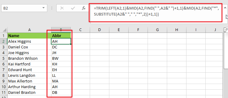
From cell A2, if you want to extract the initials, enter this formula in cell B2.

=TRIM(LEFT(A2,1)&MID(A2,FIND(" ",A2&" ")+1,1)&MID(A2,FIND("*",SUBSTITUTE(A2&" "," ","*",2))+1,1))

Here the text string is the string you want to extract the first letters of each word.

When you press the Enter key, all of the first letters of each word in cell A2 are retrieved.

Explanation:

1. The TRIM function eliminates any extra spaces from the text string.
2. The LEFT(A2,1) function retrieves the first letter of the text string.
3. MID(A2,FIND(” “,A2&” “)+1,1) retrieves the initial letter of the second word separated by a space.
4. MID(A2,FIND(“*”,SUBSTITUTE(A2&” “,” “,”*,”2))+1,1) retrieves the initial letter of the third word separated by a space.

NOTE:

This formula only works when three or fewer words are in a cell. You can modify ” “ in the formula to different delimiters.

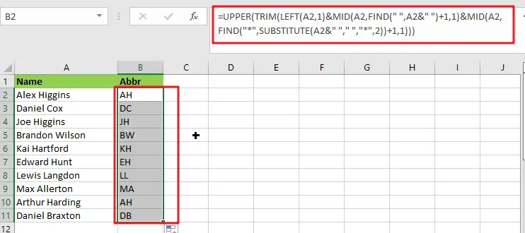
This formula extracts the initial characters in a case-insensitive manner; if you want the formula to always return in the upper case, include the UPPER function in the formula.

=UPPER(TRIM(LEFT(A2,1)&MID(A2,FIND(" ",A2&" ")+1,1)&MID(A2,FIND("*",SUBSTITUTE(A2&" "," ","*",2))+1,1)))

Related Functions

• Excel IF function
  The Excel IF function perform a logical test to return one value if the condition is TRUE and return another value if the condition is FALSE. The IF function is a build-in function in Microsoft Excel and it is categorized as a Logical Function.The syntax of the IF function is as below:= IF (condition, [true_value], [false_value])….
• Excel TEXTJOIN function
  The Excel TEXTJOIN function joins two or more text strings together and separated by a delimiter. you can select an entire range of cell references to be combined in excel 2016.The syntax of the TEXTJOIN function is as below:= TEXTJOIN  (delimiter, ignore_empty,text1,[text2])…
• Excel ROW function
  The Excel ROW function returns the row number of a cell reference.The ROW function is a build-in function in Microsoft Excel and it is categorized as a Lookup and Reference Function.The syntax of the ROW function is as below:= ROW ([reference])….
• Excel MID function
  The Excel MID function returns a substring from a text string at the position that you specify.The syntax of the MID function is as below:= MID (text, start_num, num_chars)…
• Excel INDIRECT function
  The Excel INDIRECT function returns the cell reference based on a text string, such as: type the text string “A2” in B1 cell, it just a text string, so you can use INDIRECT function to convert text string as cell reference….
• Excel MATCH  function
  The Excel MATCH function search a value in an array and returns the position of that item.The MATCH function is a build-in function in Microsoft Excel and it is categorized as a Lookup and Reference Function.The syntax of the MATCH function is as below:= MATCH  (lookup_value, lookup_array, [match_type])….
• Excel ISNUMBER function
  The Excel ISNUMBER function returns TRUE if the value in a cell is a numeric value, otherwise it will return FALSE.The syntax of the ISNUMBER function is as below:= ISNUMBER (value)…
• Excel CODE function
  The Excel CODE function returns the numeric ASCII value for the first character of a text string.The syntax of the CODE function is as below:= CODE  (text)…
• Excel LEN function
  The Excel LEN function returns the length of a text string (the number of characters in a text string).The LEN function is a build-in function in Microsoft Excel and it is categorized as a Text Function.The syntax of the LEN function is as below:= LEN(text)…
• Excel LEFT function
  The Excel LEFT function returns a substring (a specified number of the characters) from a text string, starting from the leftmost character.The LEFT function is a build-in function in Microsoft Excel and it is categorized as a Text Function.The syntax of the LEFT function is as below:= LEFT(text,[num_chars])…t)…
• Excel FIND function
  The Excel FIND function returns the position of the first text string (sub string) within another text string.The syntax of the FIND function is as below:= FIND(find_text, within_text,[start_num])…
• Excel TRIM function
  The Excel TRIM function removes all spaces from text string except for single spaces between words.  You can use the TRIM function to remove extra spaces between words in a string.The syntax of the TRIM function is as below:= TRIM (text)….