VLOOKUP is one of the key functions among all lookup & reference functions in Excel. Today we will show you the application of VLOOKUP function when there are two lookup tables.
EXAMPLE
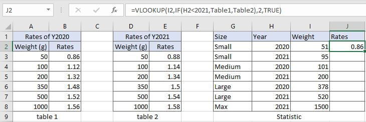
Table1 and table2 record the rates of Y2020 and Y2021 separately. Rates are increased in Y2021. In “Statistic” table, we want to fill rates information into J column based on entered “Year” information (in H column) and “Weight” information (in I column).
ANALYSIS
In this instance, there are two conditions “Year” and “Weight” to determine which value should be returned. As there are two tables showing the relationship between weight and rates on two different years, so it is equivalent to there are two lookup tables we can refer to. When performing VLOOKUP function to retrieve date, we need to know which table we will refer to.
To fix our problem, we can use IF function here to control which table will be used and delivered to VLOOKUP function as its table array. If entered year is equal to 2020, table1 will be used; if entered year is 2021, table2 will be used; so we can create a logical test that if entered year is less than 2021, then table1 is returned, otherwise table2 is returned.
As table1 or table2 only displays the weigh breaks instead of displaying each weight. So, VLOOKUP function will perform an approximate match to find out the proper weight break which entered weight belongs to.
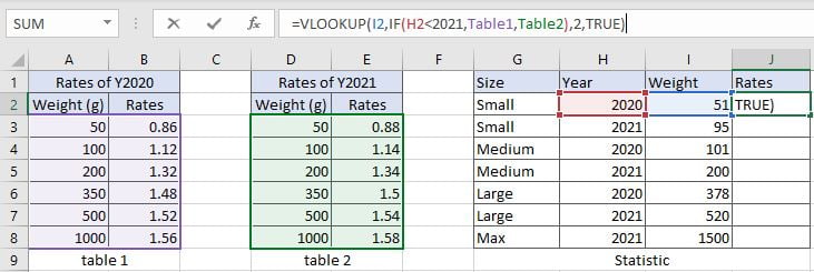
Above all, we set up VLOOKUP with IF function inside:
=VLOOKUP(I2,IF(H2<2021,Table1,Table2),2,TRUE)
// Name range A3:B8 to table1, range D3:E8 to table2.
FORMULA
Input formula =VLOOKUP(I2,IF(H2<2021,Table1,Table2),2,TRUE) into J2, press ENTER, verify that “0.86” belongs to Y2020 rates is returned properly.
Values in “Weight” column are the starting weight for each weight break. Refer to normal approximate match rules, rates “0.86” is corresponding to weight band “50-99g”, and it is from table1 of Y2020, so for small size in Y2020 with weight “51”, VLOOKUP returns 0.86. More details please see below Explanation part.
Construction of VLOOKUP function:
FUNCTION INTRODUCTION
a. VLOOKUP function looks up the input value from the first column of the given table, and returns the value we want from a particular position (row number depends on the row of lookup value, column number depends on the input argument col_index_num).
Syntax:
=VLOOKUP(lookup_value, table_array, col_index_num,[range_lookup])
For argument “range_lookup”, there are two matching modes “True” and “False”.
- The default mode is “True”, so if this optional argument is omitted, this value is set to “True” automatically.
- If we set “range_lookup” to “True”, VLOOKUP function performs an approximate match.
- If we set “range_lookup” to “False”, VLOOKUP function looks up data restrictively by performing an exact match. If look up value is not found in table, formula returns error “#N/A”.
b. IF function returns “true value” or “false value” based on the result of provided logical test. It is one of the most popular function in Excel.
Syntax:
=IF(logical_test,[value_if_true],[value_if_false])
EXPLANATION
=VLOOKUP(I2,IF(H2<2021,Table1,Table2),2,TRUE)
lookup_value is weight “51” in I2
table_array is based on the result of IF function
col_index_num is 2. Because rates are saved in the second column of table1 and table2.
range_lookup is set to TRUE. VLOOKUP function performs an approximate match.
a. There are two lookup tables in this instance. Which table is used by VLOOKUP as lookup table is controlled by IF function. If entered year in H column is 2020, it is less than 2021, table1 is returned as true result, VLOOKUP function scans lookup value from the first column of table1; if entered year is 2021, the logical test returns false, IF function delivers table2 to VLOOKUP function, then VLOOKUP scans values from the first column of table2 to find out lookup value.
b. In this formula, the lookup value is “51” in I2, year in H2 is “2020”, VLOOKUP scans “51” from the first column of table1 (A3:B8). It continues scanning until it meets the value that is greater than the lookup value. In this instance, VLOOKUP function will stop scanning when meeting “100” and returns to previous row of 50g (row3).
c. As “Rates” column is the second column in lookup table, so we enter 2 for argument col_index_num. VLOOKUP function retrieves data at the intersection of row3 and column2, so value in B3 is returned after performing VLOOKUP function.
Related Functions
- Excel INDEX function
The Excel INDEX function returns a value from a table based on the index (row number and column number)The INDEX function is a build-in function in Microsoft Excel and it is categorized as a Lookup and Reference Function.The syntax of the INDEX function is as below:= INDEX (array, row_num,[column_num])… - Excel VLOOKUP function
The Excel VLOOKUP function lookup a value in the first column of the table and return the value in the same row based on index_num position.The syntax of the VLOOKUP function is as below:= VLOOKUP (lookup_value, table_array, column_index_num,[range_lookup])….
- Excel IF function
The Excel IF function perform a logical test to return one value if the condition is TRUE and return another value if the condition is FALSE. The IF function is a build-in function in Microsoft Excel and it is categorized as a Logical Function.The syntax of the IF function is as below:= IF (condition, [true_value], [false_value])….