This post will guide you how to vlookup a value and then return multiple corresponding values horizontally in Excel. How do I lookup a value and return multiple matched values in the same row in Excel. Or how to return multiple values with VLOOKUP function in Excel.
Table of Contents
1. VLOOKUP Return Multiple Values Horizontally
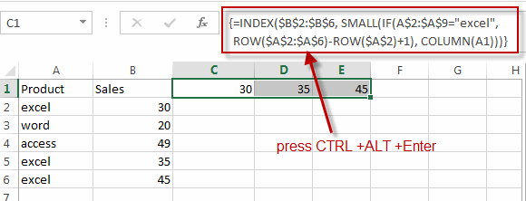
Assuming that you have a list of data that contain product name and product sales in the range A1:B6, and you want to vlookup a product “excel”” and return all sales value of the “excel” horizontally.
We have talked that the VLOOKUP function can be used to return only a corresponding value of the first occurrence of a lookup value. And if you want to return multiple values horizontally, how to achieve it.
You can create a complex array formula based on the INDEX function, the SMALL function, the IF function, the ROW function and the COLUMN function.
=INDEX($B$2:$B$6, SMALL(IF(A$2:$A$9="excel", ROW($A$2:$A$6)-ROW($A$2)+1), COLUMN(A1)))Type this formula into a blank cell and then press Ctrl+Alt+Enter shortcuts to change this formula as array formula. And then drag the AutoFill handle from Cell C1 to E1.

You will see that the multiple values have been extracted into the same row.
2. VLOOKUP Return Multiple Values Horizontally using VBA
let’s explore the second method—a more personalized approach using a User Defined Function with VBA code.
Press Alt + F11 to open the Visual Basic for Applications (VBA) editor.
In the editor, go to Insert > Module to add a new module.
Copy and paste the provided VBA code into the module.
Function VLOOKUPMultiple(lookupValue As Variant, tableRange As Range) As Variant
    Dim resultArray() As Variant
    Dim rowIndex As Long
    Dim colIndex As Long
    Dim count As Long

    count = 0

    For rowIndex = 1 To tableRange.Rows.count
        If tableRange.Cells(rowIndex, 1).Value = lookupValue Then
            count = count + 1
        End If
    Next rowIndex

    If count > 0 Then
        ReDim resultArray(1 To 1, 1 To count)

        count = 0

        For rowIndex = 1 To tableRange.Rows.count
            If tableRange.Cells(rowIndex, 1).Value = lookupValue Then
                count = count + 1
                resultArray(1, count) = tableRange.Cells(rowIndex, 2).Value
            End If
        Next rowIndex

        VLOOKUPMultiple = resultArray
    Else
        VLOOKUPMultiple = CVErr(xlErrNA)
    End If
End Function
Close the VBA editor.
Return to your Excel workbook.
select D1, E1, F1 simultaneously, type :
=VLOOKUPMultiple("excel", A$2:B$6)Press Ctrl + Shift + Enter to apply the formula as an array formula.
Observe as the VBA code dynamically returns multiple values horizontally for each occurrence of the LookupValue, and they are displayed in cells D1, E1, F1, and so forth.
Now, by using Ctrl + Shift + Enter, you’ll successfully display the array result into different cells, allowing you to visualize the multiple sales values corresponding to each occurrence of the LookupValue “excel” in Range A2:A6. Adjust the range and LookupValue as needed for your data.
3. Video: VLOOKUP Return Multiple Values Horizontally
Welcome to an Excel video tutorial where we explore the art of VLOOKUP returning multiple values horizontally. In this session, we’ll uncover two effective methods—one harnessing the power of Excel formulas using the INDEX and SMALL functions, and the other delving into a User Defined Function (UDF) with VBA code.
3. Related Functions
- Excel SMALL function
The Excel SMALL function returns the smallest numeric value from the numbers that you provided. Or returns the smallest value in the array.The syntax of the SMALL function is as below:=SMALL(array,nth) … - Excel INDEX function
The Excel INDEX function returns a value from a table based on the index (row number and column number)The INDEX function is a build-in function in Microsoft Excel and it is categorized as a Lookup and Reference Function.The syntax of the INDEX function is as below:= INDEX (array, row_num,[column_num])… - Excel ROW function
The Excel ROW function returns the row number of a cell reference.The ROW function is a build-in function in Microsoft Excel and it is categorized as a Lookup and Reference Function.The syntax of the ROW function is as below:= ROW ([reference])…. - Excel IF function
The Excel IF function perform a logical test to return one value if the condition is TRUE and return another value if the condition is FALSE. The IF function is a build-in function in Microsoft Excel and it is categorized as a Logical Function.The syntax of the IF function is as below:= IF (condition, [true_value], [false_value])…. - Excel COLUMN function
The Excel COLUMN function returns the first column number of the given cell reference.The syntax of the COLUMN function is as below:=COLUMN ([reference])…. - Excel VLOOKUP function
The Excel VLOOKUP function lookup a value in the first column of the table and return the value in the same row based on index_num position.The syntax of the VLOOKUP function is as below:= VLOOKUP (lookup_value, table_array, column_index_num,[range_lookup])….
Leave a Reply
You must be logged in to post a comment.