VLOOKUP is one of the key functions among all lookup & reference functions in Excel. It can scan and retrieve data from a static or dynamic table based on your lookup value. It can perform approximate match or exact match by setting lookup matching modes.
Today, we will show you the way to apply VLOOKUP function to retrieve data from lookup table on another worksheet. It is similar to applying VLOOKUP formula to retrieve data on the same worksheet. In our daily work, we often need to extract data from another worksheet using VLOOKUP function, if this is a confusing question for you, today’s article will help you to solve your problem.
EXAMPLE
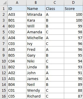
Table1: This table is located in sheet “All Classes”.
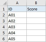
Table2: This table is located in sheet “Class A”. Table1 and table2 are in the same workbook.
In this example, we want to get score from “Score” column of table1 in sheet “All Classes” to fill “Score” column of table2 in sheet “Class A” correspondingly.
We can see that table1 is a summary and all IDs from table2 can be found in this table. Besides, they both list ID as the first column. So, we can apply VLOOKUP function to perform an exact match lookup to get score for each student properly.
ANALYSIS
This is a typical example that can be solved by VLOOKUP function. Unlike basic VLOOKUP examples, in this instance, for class A, ID and scores are not displayed in the same table, scores are only listed in the last column of table on another worksheet, and this table is our lookup table. To retrieve data from lookup table on another worksheet, we just need to add ‘sheet name’! before range reference.
Actually, when typing VLOOKUP the second argument “table_array”, you can directly move to the worksheet you can find your lookup table (then this worksheet is displayed on top), drag and drop the lookup table, then ‘sheet name’! with range reference is entered automatically and shown in the formula bar properly.
We create below formula with VLOOKUP for this instance:
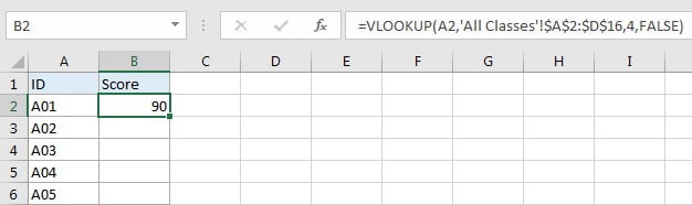
=VLOOKUP(A2,'All Classes'!$A$2:$D$16,4,FALSE)
FORMULA
Input formula =VLOOKUP(A2,’All Classes’!$A$2:$D$16,4,FALSE) into B2, press ENTER, verify that score “90” is returned by formula properly for ID A01.
FUNCTION INTRODUCTION
a. VLOOKUP function looks up the input value from the first column of the given table, and returns the value we want from a particular position (row number depends on the row of lookup value, column number depends on the input argument col_index_num).
Syntax:
=VLOOKUP(lookup_value, table_array, col_index_num,[range_lookup])
For argument “range_lookup”, there are two matching modes “True” and “False”.
- The default mode is “True”, so if this optional argument is omitted, this value is set to “True” automatically.
- If we set “range_lookup” to “True”, VLOOKUP function performs an approximate match.
- If we set “range_lookup” to “False”, VLOOKUP function looks up data restrictively by performing an exact match. If look up value is not found in table, formula returns error “#N/A”.
EXPLANATION
=VLOOKUP(A2,'All Classes'!$A$2:$D$16,4,FALSE)
lookup_value is input into A2 (ID “A01”)
table_array is ‘All Classes’!$A$2:$D$16
col_index_num is 4. Because scores are saved in the fourth column of this table.
range_lookup is set to FALSE. VLOOKUP function performs an EXACT match.
a. In this formula, the look up value is “A01”, VLOOKUP scans this value from the first column of table in worksheet “All Classes”. It continues scanning until it meets the value that is exactly the same with lookup value. In this case, VLOOKUP function will stop scanning when meeting “A01” and stay in current row.
b. Table array is ‘All Classes’!$A$2:$D$16, this table contains lookup value in its first column and expected value in its last column. We add “$” before row and column to lock this range, so when copying down the formula, the range doesn’t change. Besides, as we mentioned before, sheet name is added before range reference, so VLOOKUP function can find out lookup table from proper worksheet.
c. As Score column is the fourth column in lookup table, so we enter 4 as col_index_num. VLOOKUP function retrieves data at the intersection of column “Score” and row “A01”.
d. We set range_lookup mode to “FALSE”, so VLOOKUP function performs an exact match lookup and this operation can make sure that VLOOKUP returns correct score for each student. If lookup ID cannot be found in the given table, an error #N/A will be returned.
Related Functions
- Excel INDEX function
The Excel INDEX function returns a value from a table based on the index (row number and column number)The INDEX function is a build-in function in Microsoft Excel and it is categorized as a Lookup and Reference Function.The syntax of the INDEX function is as below:= INDEX (array, row_num,[column_num])… - Excel VLOOKUP function
The Excel VLOOKUP function lookup a value in the first column of the table and return the value in the same row based on index_num position.The syntax of the VLOOKUP function is as below:= VLOOKUP (lookup_value, table_array, column_index_num,[range_lookup])….