VLOOKUP is one of the key functions among all lookup & reference functions in Excel. It can scan and retrieve data from a static or dynamic table based on your lookup value. It can perform approximate match or exact match by setting lookup matching modes.
Today, we will show you the way to apply VLOOKUP to retrieve data by date. In our daily work, as sales or other items are often sorted by date, so we often need to retrieve data by date. If this is a confusing question for you, today’s article will help you to solve your problem.
Table of Contents
EXAMPLE
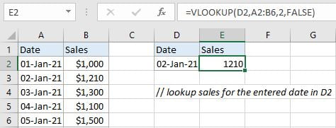
In this instance, we want to know the corresponding sales for the entered date “02-Jan-21” in D2. We can see that the entered date “02-Jan-21” can be found in “Date” column of the table on the left side (range A2:B6). And sales for different dates are also recorded in this table. Besides, for both two tables, “Dates” are listed in the first column and “Sales” are listed in the second column, they have the same table structure. So, table on the left side is our lookup table in this instance.
We can create formula with VLOOKUP function to solve this problem. This is a standard usage of VLOOKUP function.
FORMULA
Input formula =VLOOKUP(D2,A2:B6,2,FALSE) into E2, press ENTER, verify that “1210” is returned properly.
FUNCTION INTRODUCTION
a. VLOOKUP function looks up the input value from the first column of the given table, and returns the value we want from a particular position (row number depends on the row of lookup value, column number depends on the input argument col_index_num).
Syntax:
=VLOOKUP(lookup_value, table_array, col_index_num,[range_lookup])
For argument “range_lookup”, there are two matching modes “True” and “False”.
- The default mode is “True”, so if this optional argument is omitted, this value is set to “True” automatically.
- If we set “range_lookup” to “True”, VLOOKUP function performs an approximate match.
- If we set “range_lookup” to “False”, VLOOKUP function looks up data restrictively by performing an exact match. If look up value is not found in table, formula returns error “#N/A”.
EXPLANATION
=VLOOKUP(D2,A2:B6,2,FALSE)
lookup_value is input into D2 (date “02-Jan-21”)
table_array is A2:B6
col_index_num is 2. Because sales are saved in the second column of this table.
range_lookup is set to FALSE. VLOOKUP function performs an EXACT match.
a. In this formula, the look up value is “02-Jan-21”, VLOOKUP scans this value from the first column of lookup table A2:B6. It continues scanning until it meets the same date. In this case, VLOOKUP function will stop scanning when meeting “02-Jan-21” in cell A3 and stay in current row.
b. As “Sales” column is the second column in lookup table, so we enter 2 as col_index_num. VLOOKUP function retrieves data at the intersection of column 2 and row 3.
c. We set range_lookup mode to “FALSE”, so VLOOKUP function performs an exact match lookup and this operation can make sure that VLOOKUP returns correct sales value for the entered date. If lookup value cannot be found in the given table, an error #N/A will be returned.
Related Functions
- Excel INDEX function
The Excel INDEX function returns a value from a table based on the index (row number and column number)The INDEX function is a build-in function in Microsoft Excel and it is categorized as a Lookup and Reference Function.The syntax of the INDEX function is as below:= INDEX (array, row_num,[column_num])… - Excel VLOOKUP function
The Excel VLOOKUP function lookup a value in the first column of the table and return the value in the same row based on index_num position.The syntax of the VLOOKUP function is as below:= VLOOKUP (lookup_value, table_array, column_index_num,[range_lookup])….