This post will guide you how to create 3d references to conditionally sum identical ranges that exist in the multiple sheets, and make it all in only one formula. How do I create a formula to sumif with 3d reference for multiple worksheet based on multiple criteria in excel.

Sumif with 3D Reference for Multiple worksheet

If you want to sum 3d references across the different worksheet, and you need to create a complex formula based on the SUMPRODUCT function, the SUMIF function, and the INDIRECT function.

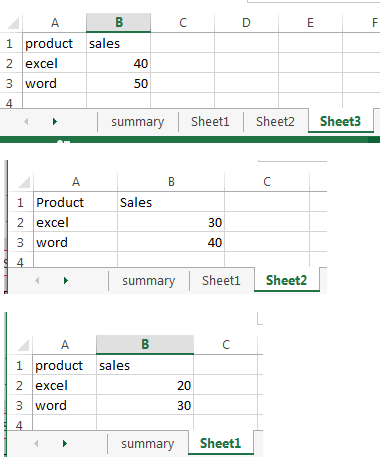
For example, you have a workbook with four worksheets (summary, sheet1,sheet2,and sheet3), and you want to create a formula in the summary worksheet to sum across the number of sales tab based on two criteria. How to achieve it. Let’s do the following steps:

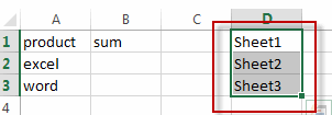
#1 create a name range “sheets” that contains multiple worksheet names(sheet1,sheet2,sheet3)

#2 switch to summary sheet, and type this formula in Cell B1 to sum the sales across name range.

=SUMPRODUCT(SUMIF(INDIRECT("'"&sheets&"'!"&"A2:A3"),A2,INDIRECT("'"&sheets&"'!"&"B2:B3")))

#3 press Enter key in your keyboard and then drag the AutoFill handler over other cell to apply this formula.

Related Functions

• Excel SUMPRODUCT function
  The Excel SUMPRODUCT function multiplies corresponding components in the given one or more arrays or ranges, and returns the sum of those products.The syntax of the SUMPRODUCT function is as below:= SUMPRODUCT (array1,[array2],…)…
• Excel SUMIF Function
  The Excel SUMIF function sum the numbers in the range of cells that meet a single criteria that you specify. The syntax of the SUMIF function is as below:=SUMIF (range, criteria, [sum_range])…
• Excel INDIRECT function
  The Excel INDIRECT function returns the cell reference based on a text string, such as: type the text string “A2” in B1 cell, it just a text string, so you can use INDIRECT function to convert text string as cell reference….