This Sales Invoice Tracker template for excel will calculate line item of invoice subtotals, sales tax, and allow you choose the different type of invoice and then display the corresponding customer invoiced data. And it is a little complicated and also very powerful template. And you can download it freely to use it in your business.

This Sales Invoice Tracker template is mainly used to maintain a history of customers, invoices and invoice details. You can analyze your previously invoiced data base on one invoice type.

Sales Invoice Tracker template Description

4 worksheets will be used in this template: Invoice, Customers, Invoices-Main, Invoice Details

Invoice#:

• select an Invoice type from the drop down list of “Invoice#“

The range B4:B5 in the worksheet “Invoices-Main” is selected as the Data source of G4 cell in “Invoice” worksheet.

If you want to check the data source, just following the below steps:

1# click “G4” cell in worksheet “Invoice”

2# click “DATA” tab in excel Ribbon, then click “Data Validation” command in “Data Tools” group

3# “Data Validation” window will appear.

4# click “Data source” button, it will locate to the referring range.

or you can check the defined name (=Invoice_No) from “FORMULAS”->”Name Manager”.

The excel formula of Customer information

All the fields of customer information apply to the similar Excel formula, as below:

The field “Bill To” ‘s formula:

=IFERROR(VLOOKUP(VLOOKUP(rngInvoice,InvoicesMain,2,FALSE),CustomerList,3,TRUE),””)

Let’s see how to understand this formula:

Assuming: the value “3-456-2” is selected in G4 cell.

rngInvoice: It’s a defined name and refers to “=Invoice!G$4”, so now rngInvoice=”3-456-2”
InvoicesMain:  It’s a defined name of a range of cell in the “Invoices-Main” worksheet and refers to “=’Invoices-Main’!$B$4:$K$5”
CustomerList:  It’s a defined name of a range of cell in the worksheet “Customers” and refers to “=Customers!$B$4:$L$5”
VLOOKUP(rngInvoice,InvoicesMain,2,FALSE): It will search “3-456-2” string in the first column of excel range “InvoicesMain”, and returns the value from column2 that is in the same row, and this excel formula will return: “2 – Contoso, Ltd”
VLOOKUP(VLOOKUP(rngInvoice,InvoicesMain,2,FALSE),CustomerList,3,TRUE) : it will search “2 – Contoso, Ltd” in the first column of excel range “CustomerList” and returns the value from column 3 that is in the same row, this excel formula will return: “Contoso, Ltd”

The excel formula of invoiced data

It mainly use array formula with INDEX, IF,SMALL and Row functions, such like below formula:

Assuming: the value “3-456-2” is selected in G4 cell.

The Cell B9’s formula:

=IFERROR(INDEX(InvoiceDetails,SMALL(IF(InvoiceDetails[Invoice '#]=rngInvoice,ROW(InvoiceDetails)-ROW(InvoiceDetails[#Headers])), ROW(1:1)), MATCH($B$8, InvoiceDetails[#Headers], 0)),"")

rngInvoice: equal to “3-456-2”
InvoiceDetails: it’s a defined name of a range of cell in the worksheet “Invoice Details” and refers to “=’Invoice Details’!$B$4:$H$40”
InvoiceDetails[Invoice ‘#]: it’s range cell and  refers to: $C$4:$C$40
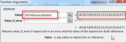
ROW(InvoiceDetails): it will return all row numbers for range InvoiceDetails(C4:C40), this function will return: “{4;5;6;…40}

 

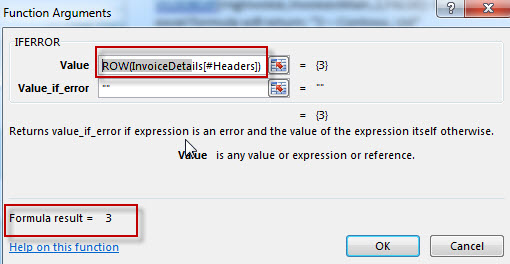
ROW(InvoiceDetails[#Headers]): it will return the row number of “headers” row in the worksheet “Invoice Details”, this function will return value:”3”

ROW(InvoiceDetails)-ROW(InvoiceDetails[#Headers]): the returned row number minus the row number of headers row. Such as: (row )29 –(row )3=(row )26
IF(InvoiceDetails[Invoice ‘#]=rngInvoice,ROW(InvoiceDetails)-ROW(InvoiceDetails[#Headers])): If the value of  “Invoice #” in the range $C$4:$C$40 equal to rngInvoice (assuming: 3-456-2), then return its row number, so this IF function will return a array list , contains all row numbers that match the condition. Such like: {26;27;28…37}
ROW(1:1): return “1”
ROW(2:2): return “2”
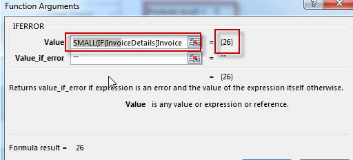
SMALL(IF(InvoiceDetails[Invoice ‘#]=rngInvoice,ROW(InvoiceDetails)-ROW(InvoiceDetails[#Headers])), ROW(1:1)): it will return the smallest value in the array list, this formula will return “26”

SMALL(IF(InvoiceDetails[Invoice ‘#]=rngInvoice,ROW(InvoiceDetails)-ROW(InvoiceDetails[#Headers])), ROW(2:2)):it will return the second smallest value in the array list, this formula will return “27”
InvoiceDetails[#Headers]: returns all values of headers row in the worksheet “Invoice Details”, such like: {“Description”,”Invoice#”, “Item#”…}
MATCH($B$8, InvoiceDetails[#Headers], 0)): it will return the position of value “Item#” in the range InvoiceDetails[#Headers]. This function will return: “3”

 So now C9’s formula can be reduce to: =IFERROR(INDEX(InvoiceDetails,26,3,””), it will return a value(Z4567) from table “InvoiceDetails” based on the index (26,3).

How To get this free Sales Invoice Tracker template in Excel?

Click “File” Tab ->”New” , then input “Sales Invoice Tracker template”  to search online template in the search box.