This post will guide you how to make a cumulative sum chart in Excel. How do I create a cumulative sum chart in Excel 2013/2016. How to add a cumulative total to a line chart in Excel.

1. Create a Cumulative Chart

Assuming that you have a list of data in range B1:C5 that contain sales data. And you want to create a cumulative sum chart for these data. How to achieve it. You just need to do the following steps:

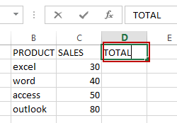
Step1: select one blank cell next to the Sales column, and type the name of column D header as “TOTAL”.

Step2: type the following formula based on the SUM function in the Cell D2. And press Enter key in your keyboard, and then drag the AutoFill Handle from Cell D2 to D5.

=SUM(C$2:C2)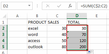

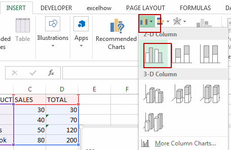
Step3: select all data, and then go to INSERT tab, click Insert Column Chart command under Charts group. And select one 2-D Clustered Column. And one Column Chart has been created based on the selected data.

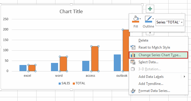
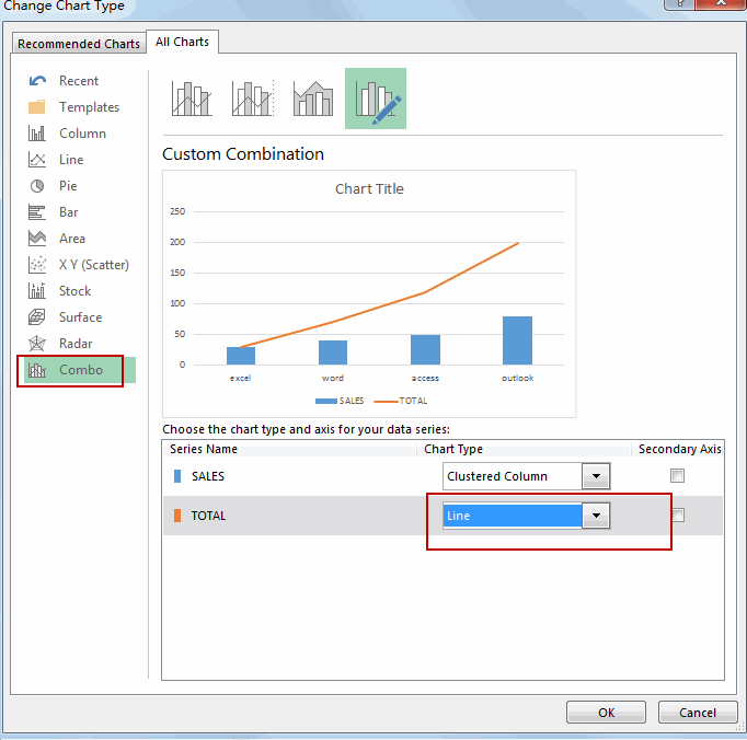
Step4: click Total Data series in the chart, and right click on it and select Change Series Chart Type from the popup menu list. The Change Chart Type dialog will open.

Step5: change the Chart type for TOTAL data series to Line, click OK button.

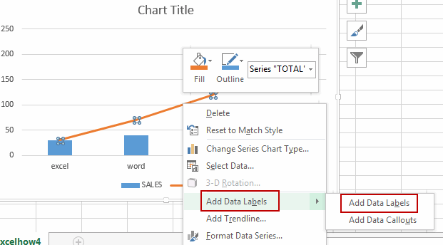
Step6: select the line data series, and right click on it. And select Add Data Labels, then select Add Data Labels sub menu.

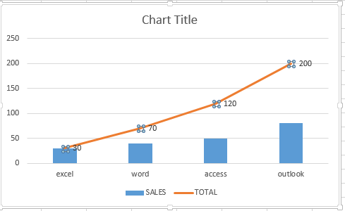
Step7: Let’s see the result.

2. Video: Make a Cumulative Chart in Excel

This video will guide you step-by-step on how to make a cumulative sum chart in Excel to visualize the running total of data.

3. Related Functions

• Excel SUM function
  The Excel SUM function will adds all numbers in a range of cells and returns the sum of these values. You can add individual values, cell references or ranges in excel.The syntax of the SUM function is as below:= SUM(number1,[number2],…)…